In Magnetic Resonance, zero filling involves artificially extending a dataset in the time domain (FID) or spatial-frequency domain (k-space) by padding it with zeros.
The Physics of Zero Filling
While it is often mistaken for increasing “true” resolution, zero filling does not add new information. According to the Fourier Shift Theorem and DFT properties:
In MRS (Time Domain): Padding the end of an FID with zeros increases the total number of points fed into the FFT. This acts mathematically as a sinc interpolation in the frequency domain, improving the digital resolution (the visual spacing between points on the x-axis) and allowing us to better define the true peak shape and position.
In MRI (k-space): Symmetrically padding the high-frequency edges of k-space decreases the apparent pixel size in the reconstructed image. This reduces truncation artifacts (Gibbs ringing) by smoothly interpolating intensity values between the original coarse pixels.
import matplotlib.pyplot as plt
import numpy as np
import xarray as xr

# Ensure the accessor is registered
import xmris
1. Generating a Realistic FID: Sampled Data
Let’s define a function to simulate a multi-component FID with decay and specific frequency offsets.
def simulate_fid(t):
    """Simulate a 3-peak FID (doublet + singlet) given a time array."""
    peak1 = 1.0 * np.exp(-t / 0.05) * np.exp(1j * 2 * np.pi * 50 * t)
    peak2 = 0.5 * np.exp(-t / 0.03) * np.exp(1j * 2 * np.pi * 30 * t)
    peak3 = 0.5 * np.exp(-t / 0.03) * np.exp(1j * 2 * np.pi * 70 * t)
    return peak1 + peak2 + peak3
We will simulate a realistic dataset with finite bandwidth.
(Note: The dwell time must be small enough to satisfy the Nyquist criterion. A 2 ms dwell time yields a 500 Hz spectral width ( Hz), safely capturing our 70 Hz peak without aliasing).
# Generate realistically Sampled data
dwell_time = 0.002
bw_sampled = 1 / dwell_time  # 500 Hz
n_points_sampled = 64
t_sampled = np.arange(n_points_sampled) * dwell_time

da_fid_sampled = xr.DataArray(
    simulate_fid(t_sampled),
    dims=["time"],
    coords={"time": t_sampled},
    attrs={"sequence": "FID", "B0": 3.0},
)
2. Time-Domain Zero Filling
We apply zero filling to the sampled data, extending it from 64 points to 512 points by padding zeros at the end of the acquisition window.
target_points = 512

# Zero fill the sampled array
da_fid_zf = da_fid_sampled.xmr.zero_fill(
    dim="time", target_points=target_points, position="end"
)

fig, ax1 = plt.subplots(figsize=(10, 4))

# Original Sampled Points
da_fid_sampled.real.plot(
    ax=ax1,
    marker="o",
    color="tab:orange",
    linestyle="-",  # Connected to show the original signal path
    label=f"Sampled ($\Delta t$={dwell_time * 1000:.1f}ms, BW={bw_sampled:.0f}Hz)",
    zorder=5,
)

# Zero-filled tail
da_fid_zf.isel(time=slice(n_points_sampled, target_points)).real.plot(
    ax=ax1, color="black", linestyle="--", alpha=0.5, label="Zero-padded Tail"
)


ax1.set_xlim(-0.01, 0.4)
ax1.set_title(f"Time Domain (Real Part) | Fixed $\Delta t$ = {dwell_time * 1000:.1f}ms")
ax1.set_ylabel("Amplitude")
ax1.legend()

plt.tight_layout()
plt.show()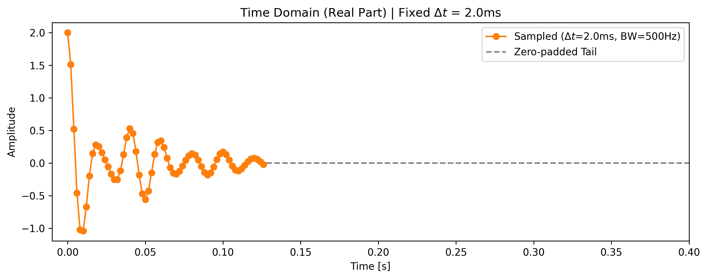
Under the Hood: No Magic Strings
As a user, you can pass simple strings like "time" and "frequency" to xmris functions. However, internally, the package never uses raw strings. It maps your input to a strict global vocabulary (xmris.core.config.DIMS and COORDS).
This architecture allows xmris to intercept your request and automatically inject physical metadata (like setting the new coordinate units to Hz or s) or properly extrapolate coordinate values when extending an array with zeros.
For more info see xmris Architecture: Why We Built It This Way
Interpolating the Truth (Frequency Domain)
When we transform the zero-filled data, the zeros act as mathematical anchors, forcing the FFT to interpolate the discrete points, resulting in a much smoother spectrum. Note that the peaks do not become narrower (resolution has not increased), but their shapes are better defined.
fig, ax2 = plt.subplots(figsize=(10, 4))

spec_sampled = da_fid_sampled.xmr.to_spectrum().real
spec_zf = da_fid_zf.xmr.to_spectrum().real

# Normalize spectra to their maximum value (peak height = 1.0)
spec_sampled_norm = spec_sampled / spec_sampled.max()
spec_zf_norm = spec_zf / spec_zf.max()

# Zero-filled Interpolation
spec_zf_norm.plot(
    ax=ax2,
    color="black",
    marker=".",
    linewidth=1.5,
    label=f"Zero-filled ({target_points} pts)",
    zorder=1,
)
# Original Sampled Points
spec_sampled_norm.plot(
    ax=ax2,
    marker="o",
    markersize=6,
    color="tab:orange",
    label=f"Sampled ({n_points_sampled} pts)",
    zorder=5,
    linestyle="", # Remove lines to emphasize the discrete nature of the raw FFT
)

cf = 50  # centerfreq
ax2.set_xlim(cf - 70, cf + 70)
ax2.axvline(cf, color="gray", zorder=-10)
ax2.set_title(
    f"Frequency Domain (Normalized) | Constant BW = {bw_sampled:.0f}Hz ($\Delta t$={dwell_time * 1000:.1f}ms)"
)
ax2.set_ylabel("Normalized Amplitude")
ax2.legend()

plt.tight_layout()
plt.show()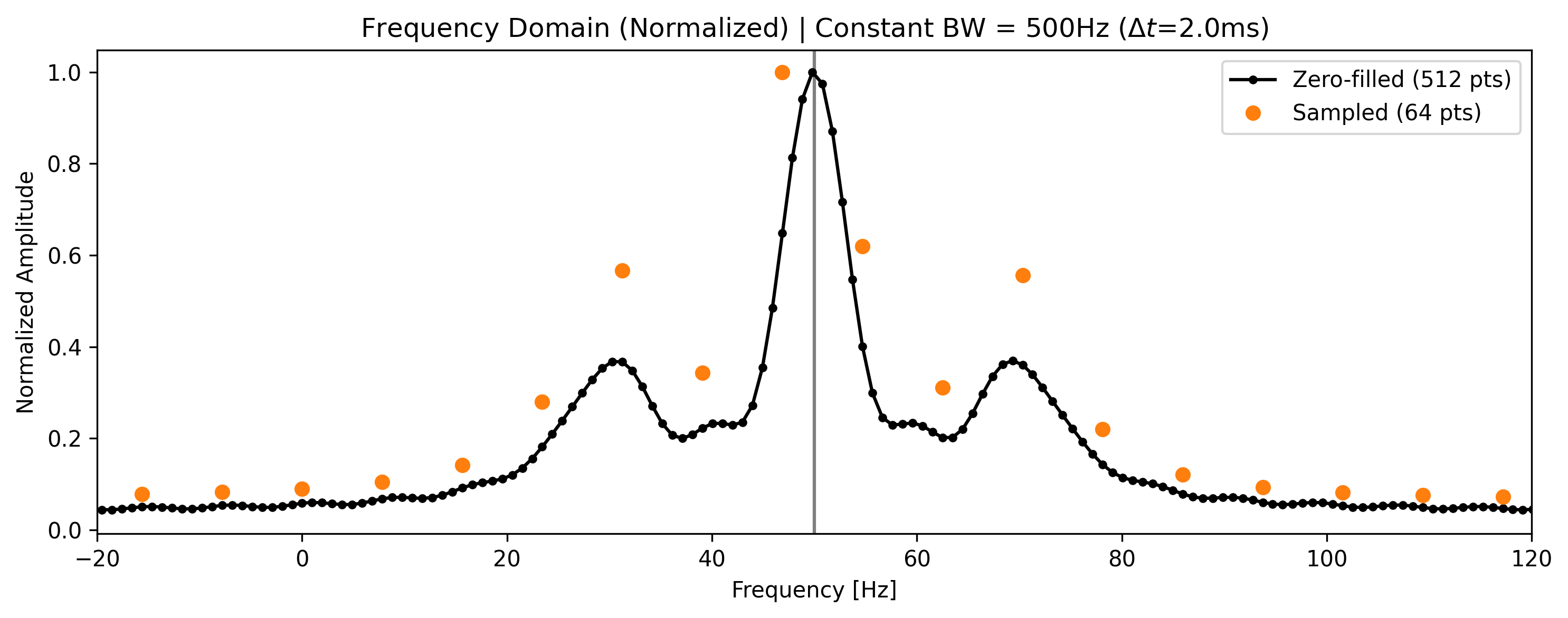
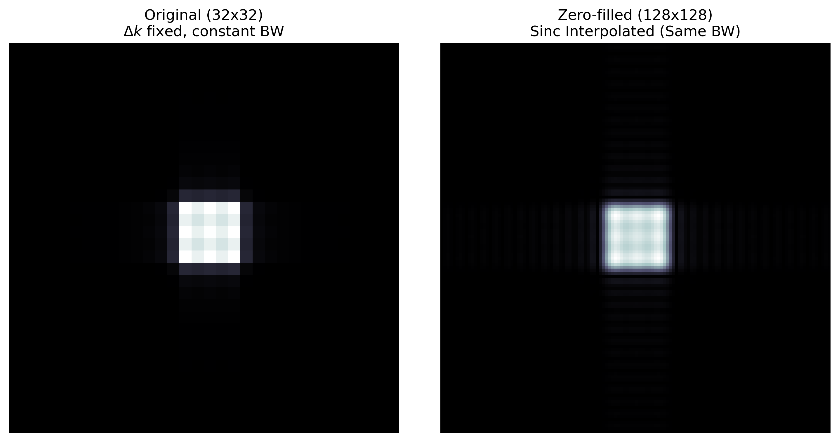
3. Spatial Frequency Zero Filling (2D K-Space)
In MRI imaging, we zero-fill k-space symmetrically to artificially boost the digital resolution matrix (e.g., from 32x32 to 128x128).
# Create a low-res 32x32 k-space grid
N = 32
k_vec = np.linspace(-N // 2, N // 2 - 1, N)
kx, ky = np.meshgrid(k_vec, k_vec)

# Physics: A rectangular object in image space is a 2D sinc in k-space
kspace_2d = np.sinc(kx / 6) * np.sinc(ky / 6)
da_k2d = xr.DataArray(
    kspace_2d + 0j, dims=["ky", "kx"], coords={"ky": k_vec, "kx": k_vec}, attrs={"domain": "k-space"}
)

# Symmetrically Zero-fill to 128x128
target_k_points = 128
da_k2d_zf = da_k2d.xmr.zero_fill(dim="kx", target_points=target_k_points, position="symmetric")
da_k2d_zf = da_k2d_zf.xmr.zero_fill(dim="ky", target_points=target_k_points, position="symmetric")
Image Reconstruction
Transforming back to image space demonstrates how zero-filling smooths the blocky pixels of the low-resolution acquisition. Because we use symmetric padding in k-space, the resulting image remains centered.
# Transform to image space (using standard centered FFT functions from xmris)
# Note: In a real xmris pipeline, we would use a dedicated spatial transform,
# but for this demonstration we will use numpy's generic ifftn/ifftshift.
img_orig = np.abs(np.fft.ifftshift(np.fft.ifftn(np.fft.fftshift(da_k2d.values))))
img_zf = np.abs(np.fft.ifftshift(np.fft.ifftn(np.fft.fftshift(da_k2d_zf.values))))

# Visualization
fig, axes = plt.subplots(1, 2, figsize=(10, 5))

axes[0].imshow(img_orig, cmap="bone", origin="lower")
axes[0].set_title(f"Original ({N}x{N})\n$\Delta k$ fixed, constant BW")

axes[1].imshow(img_zf, cmap="bone", origin="lower")
axes[1].set_title(f"Zero-filled ({target_k_points}x{target_k_points})\nSinc Interpolated (Same BW)")

for ax in axes:
    ax.axis("off")

plt.tight_layout()
plt.show()