title: Spectrum - Coordinate Transformations (Hz to ppm)¶

import matplotlib.pyplot as plt
import matplotlib_inline.backend_inline

# 1. Use retina for crisp, PDF-like text that never disappears in HTML
matplotlib_inline.backend_inline.set_matplotlib_formats("retina")

# 2. Set a high baseline DPI
plt.rcParams["figure.dpi"] = 150

In Magnetic Resonance Spectroscopy (MRS), spectra are initially reconstructed in the frequency domain, measured in Hertz (Hz). This relative frequency axis ( $\Delta \nu$ ) is strictly dependent on the hardware—specifically, the strength of the main magnetic field ( $B_0$ ).

To compare spectra across different scanners (e.g., 1.5T vs 3T vs 7T), we convert this hardware-dependent axis into a hardware-independent axis called chemical shift, measured in parts-per-million (ppm).

xmris provides dedicated methods to swap between these coordinate systems seamlessly while tracking the physical metadata.

The Physics & Math¶

The conversion relies on two critical pieces of metadata that must be stored in your xarray.DataArray.attrs:

reference_frequency: The Larmor frequency of the target nucleus (in MHz).
carrier_ppm: The absolute chemical shift located exactly at the center of your acquisition band (0 Hz). For $^1$ H MRS, this is typically the water resonance at 4.7 ppm.

The mathematical relationships are defined as:

\text{ppm} = \text{carrier\_ppm} + \left( \frac{\text{Hz}}{\text{reference\_frequency}} \right)

(1)

\text{Hz} = (\text{ppm} - \text{carrier\_ppm}) \times \text{reference\_frequency}

(2)

import matplotlib.pyplot as plt
import numpy as np
import xarray as xr

# Ensure the accessor is registered
import xmris

1. Generating a Synthetic Spectrum¶

Let’s generate a mock frequency-domain spectrum (in Hz) acquired on a 3T scanner. We must stamp the required physics metadata into the .attrs.

# Simulated acquisition parameters for 3T
mhz = 127.7  # 1H resonance frequency at 3T
carrier = 4.7 # Transmitter centered on water
n_points = 1024
sw_hz = 2000.0 # 2 kHz spectral width

# Generate relative Hz coordinates centered at 0
hz_coords = np.linspace(-sw_hz/2, sw_hz/2, n_points)

# Simulate two peaks: Water (at 0 Hz / 4.7 ppm) and NAA (at roughly -345 Hz / 2.0 ppm)
water_peak = 1.0 / (1 + ((hz_coords - 0) / 10)**2)
naa_peak = 0.5 / (1 + ((hz_coords - (-345)) / 8)**2)
spec_data = water_peak + naa_peak

# Xarray construction with strictly required attrs
da_freq = xr.DataArray(
    spec_data,
    dims=["frequency"],
    coords={"frequency": hz_coords},
    attrs={
        "reference_frequency": mhz,
        "carrier_ppm": carrier,
        "sequence": "PRESS"
    }
)

fig, ax = plt.subplots(figsize=(8, 3))
da_freq.plot(ax=ax)
ax.set_title("Spectrum in Relative Frequency (Hz)")
ax.set_xlabel("Frequency [Hz]")
# Note: In MRS, frequency/ppm axes are traditionally plotted right-to-left
ax.invert_xaxis()
plt.show()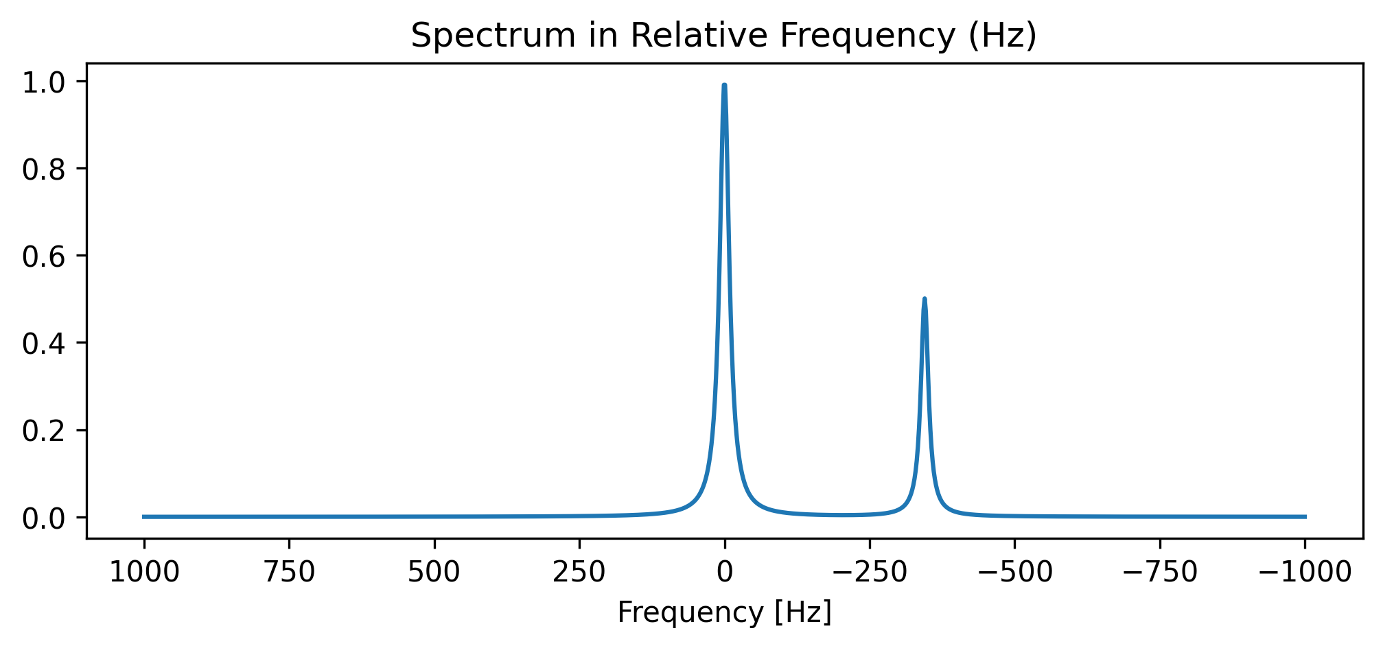

2. Converting to Chemical Shift (ppm)¶

Using .xmr.to_ppm(), xmris calculates the new chemical shift coordinates, creates a properly labeled axis, and automatically swaps the primary dimension of the DataArray from "frequency" to "chemical_shift".

# Convert to ppm using the dimension name as a plain string
da_ppm = da_freq.xmr.to_ppm(dim="frequency")

fig, ax = plt.subplots(figsize=(8, 3))
da_ppm.plot(ax=ax, color="tab:green")
ax.set_title("Spectrum in Absolute Chemical Shift (ppm)")
ax.set_xlabel("Chemical Shift [ppm]")
ax.invert_xaxis()
plt.show()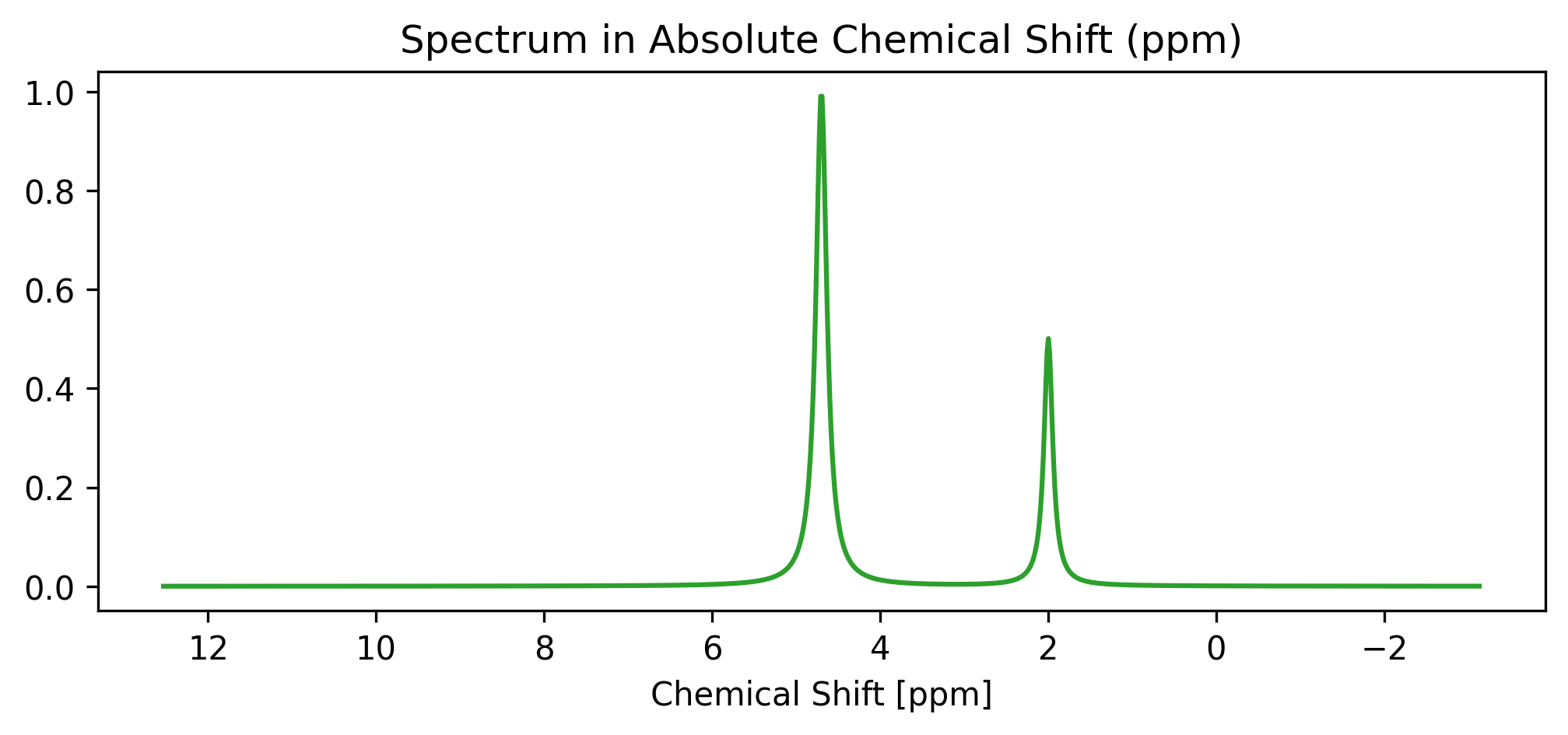

Notice how the water peak is now correctly centered at 4.7 ppm, and the NAA peak is positioned around 2.0 ppm.

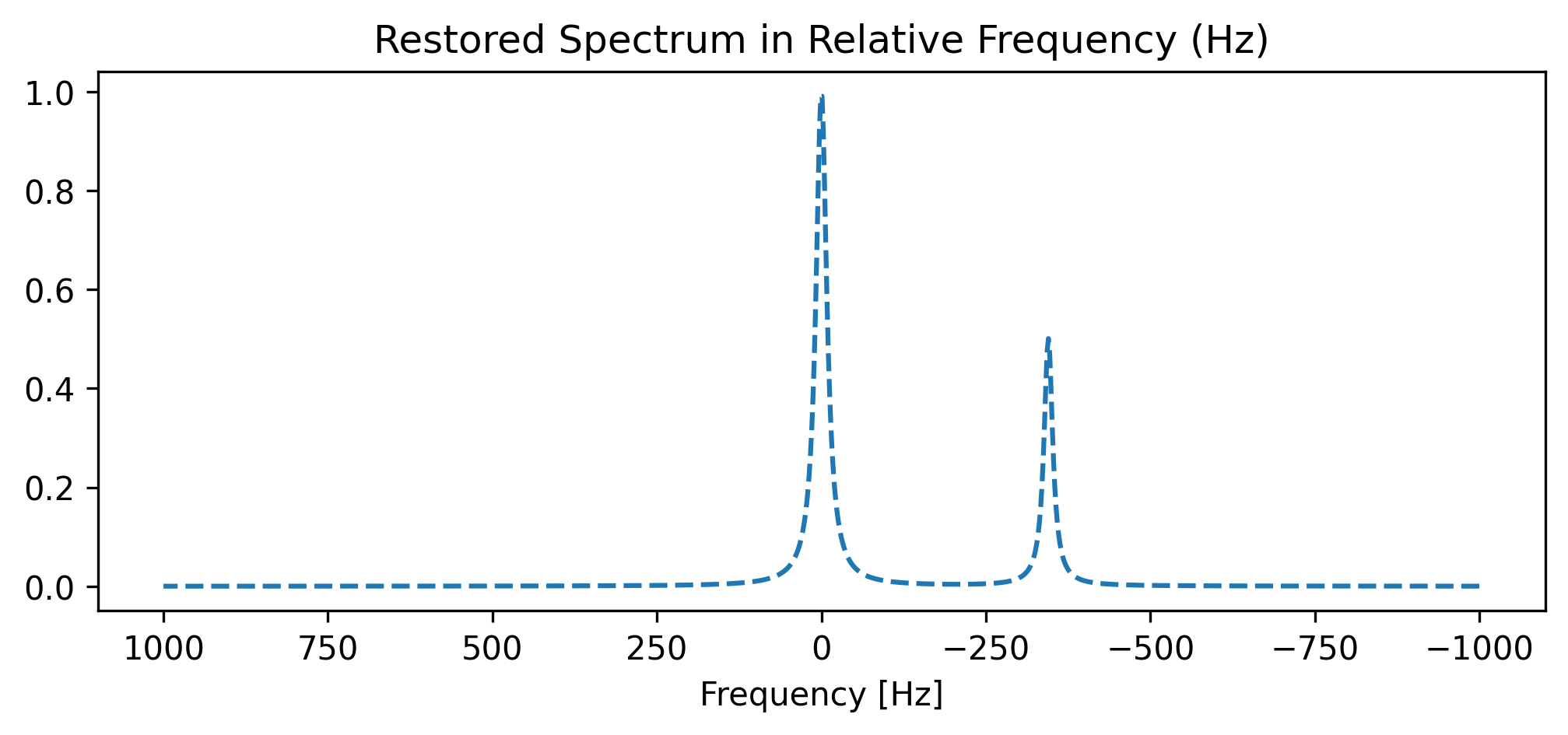
3. Converting back to Frequency (Hz)¶

The operation is perfectly invertible using .xmr.to_hz().

Because xmris preserves data lineage, the metadata attributes are completely untouched during the first transformation, meaning the DataArray has everything it needs to reconstruct the original Hz axis.

# Convert back to relative frequency (Hz)
da_hz_restored = da_ppm.xmr.to_hz(dim="chemical_shift")

fig, ax = plt.subplots(figsize=(8, 3))
da_hz_restored.plot(ax=ax, color="tab:blue", linestyle="--")
ax.set_title("Restored Spectrum in Relative Frequency (Hz)")
ax.set_xlabel("Frequency [Hz]")
ax.invert_xaxis()
plt.show()

# STRICT TESTS: Coordinate Transformations

# 1. Test to_ppm math and structural integrity
_mhz = da_freq.attrs["reference_frequency"]
_carrier = da_freq.attrs["carrier_ppm"]
_hz_vals = da_freq.coords["frequency"].values

_expected_ppm = _carrier + (_hz_vals / _mhz)

np.testing.assert_allclose(
    da_ppm.coords["chemical_shift"].values, _expected_ppm,
    err_msg="to_ppm math failed."
)
assert da_ppm.dims == ("chemical_shift",), "Dimension swap to chemical_shift failed."
assert "chemical_shift" in da_ppm.coords, "Coordinate assignment failed."
assert da_ppm.attrs == da_freq.attrs, "Attributes were dropped during to_ppm."

# 2. Test to_hz math and structural invertibility
_ppm_vals = da_ppm.coords["chemical_shift"].values
_expected_hz = (_ppm_vals - _carrier) * _mhz

np.testing.assert_allclose(
    da_hz_restored.coords["frequency"].values, _expected_hz,
    err_msg="to_hz math failed."
)
assert da_hz_restored.dims == ("frequency",), "Dimension swap back to frequency failed."
assert "frequency" in da_hz_restored.coords, "Coordinate restoration failed."

# 3. Test absolute invertibility
np.testing.assert_allclose(
    da_hz_restored.values, da_freq.values,
    err_msg="Data values altered during cycle."
)
np.testing.assert_allclose(
    da_hz_restored.coords["frequency"].values, da_freq.coords["frequency"].values,
    err_msg="Original Hz coords not perfectly restored."
)