In Magnetic Resonance Spectroscopy (MRS), the raw data acquired by the scanner is a time-domain Free Induction Decay (FID).
To visualize the chemical resonances, this digital FID signal is processed by a discrete Fourier transformation (DFT) to produce a digital MR spectrum. Because an FID conventionally starts at , we perform a standard Fast Fourier Transform (FFT) followed by a frequency-domain shift (fftshift) to center the zero-frequency (DC) component.
import matplotlib.pyplot as plt
import numpy as np
import xarray as xr

# Ensure the accessor is registered
import xmris.core.accessor
1. Generate a Synthetic FID
Let’s create an FID with two distinct resonances (at 50 Hz and -150 Hz).
Source
n_points = 1024
dwell_time = 0.001  # 1 ms dwell time implies a spectral width of 1000 Hz
t = np.arange(n_points) * dwell_time

# Two peaks with different frequencies and decay rates
peak1 = np.exp(-t / 0.05) * np.exp(1j * 2 * np.pi * 50 * t)
peak2 = 0.5 * np.exp(-t / 0.03) * np.exp(1j * 2 * np.pi * -150 * t)

da_fid = xr.DataArray(
    peak1 + peak2,
    dims=["time"],
    coords={"time": t},
    attrs={"units": "a.u.", "sequence": "FID", "B0": 3.0},
)

da_fid.real.plot(figsize=(8, 3))
plt.title("Synthetic FID (Real Part)")
plt.show()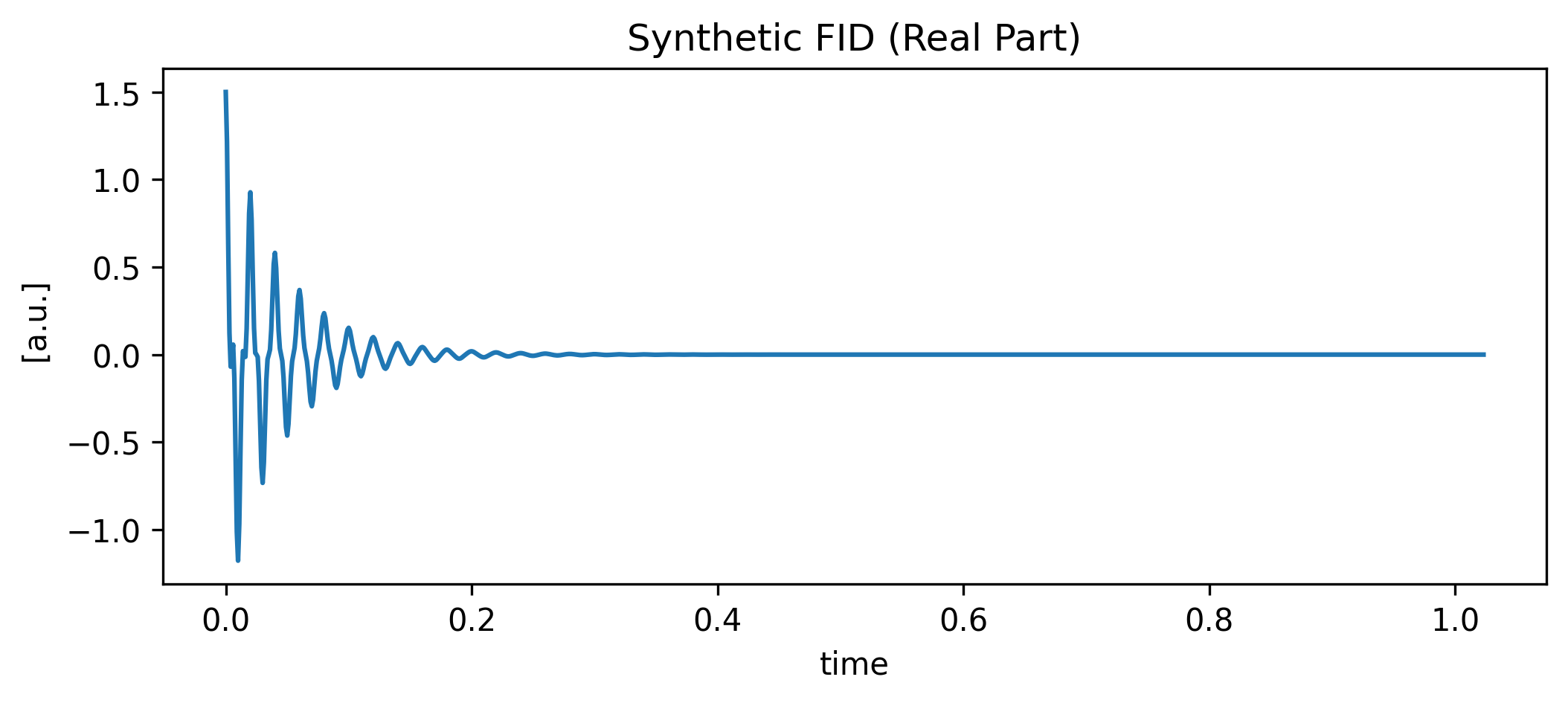
2. Convert to Spectrum
We use .xmr.to_spectrum() to perform the FFT and automatically rename the dimension to “frequency”. Notice how the resulting coordinates automatically represent the correct centered frequency axis (ranging from -500 Hz to 500 Hz).
da_spec = da_fid.xmr.to_spectrum(dim="time", out_dim="frequency")

# Plot the magnitude spectrum
np.abs(da_spec).plot(figsize=(8, 3))
plt.title("MR Spectrum (Magnitude)")
plt.xlim(250, -250)  # Standard MRS convention: reverse x-axis
plt.show()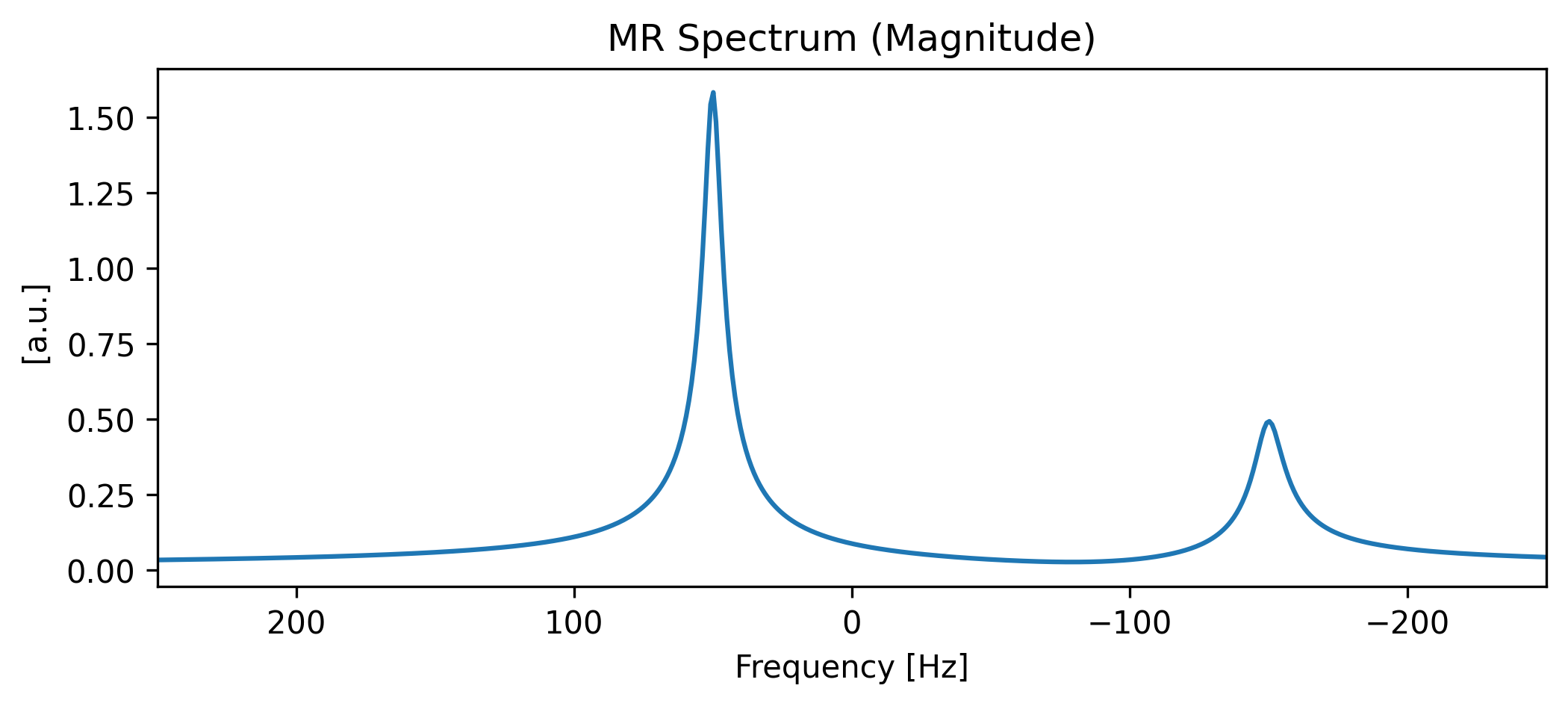
Where did that clean “Frequency [Hz]” xlabel come from?
If you spotted that our spectrum has a clean “Frequency [Hz]” xaxis label — even though we never manually assigned it (e.g. with ax.set_xlabel(...)) — good eye!
While you can pass simple strings like "time" and "frequency" to xmris functions to keep the entry barrier low, the package internally maps your input against a strict global vocabulary (xmris.core.config.DIMS and COORDS).
When .xmr.to_spectrum() built the new frequency axis, it intercepted your "frequency" string, fetched the associated physical metadata (long_name="Frequency", units="Hz"), and injected it directly into the new xarray coordinates. When you call .plot(), xarray automatically detects this metadata and formats the axis labels for you!
Bonus: Because "time" and "frequency" are declared default dimensions in xmris, we could actually drop the arguments completely and just call da_fid.xmr.to_spectrum() for the exact same result!
For more info on this design, see xmris Architecture: Why We Built It This Way
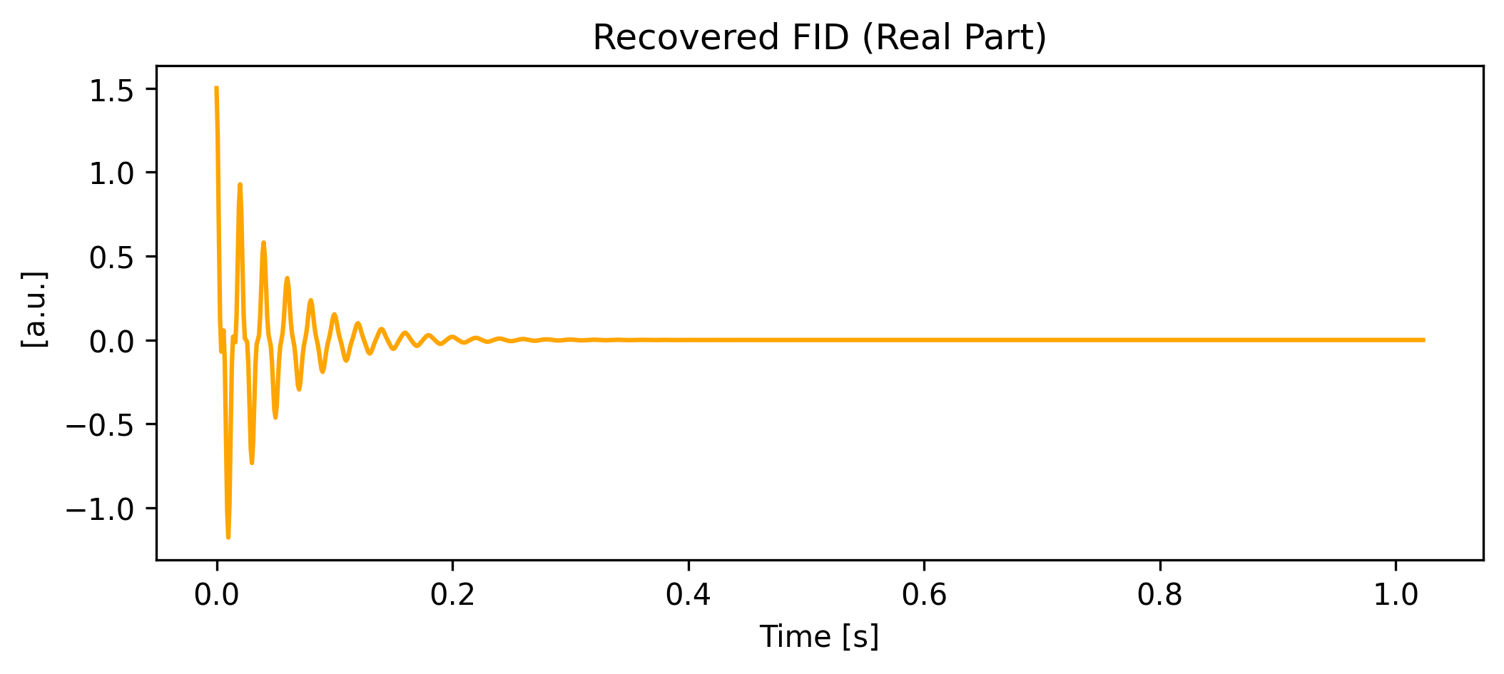
3. Convert back to FID
We can accurately recover the original time-domain signal using .xmr.to_fid().
da_recovered = da_spec.xmr.to_fid(dim="frequency", out_dim="time")

da_recovered.real.plot(figsize=(8, 3), linestyle="-", color="orange")
plt.title("Recovered FID (Real Part)")
plt.show()