In MRI and MRS, we constantly move between the time domain and frequency domain, or between -space and image space.
While numpy.fft is incredibly fast, applying it directly to physical data is notoriously finicky: it places the zero-frequency (DC) component at the edges, requiring manual fftshift operations, and it scales the signal amplitude by the number of points, breaking energy conservation (Parseval’s theorem) between domains.
The xmris Fourier module provides a mathematically rigorous, xarray-native toolbox to solve these issues. It handles orthogonal normalization, coordinate math, and shifting automatically.
Overview of Available Functions
The module provides three pairs of functions to handle any transformation scenario:
Pure Transforms (
fft/ifft):Performs orthogonal, N-dimensional transforms with no shifting. Perfect for signals that strictly start at .
Explicit Shifts (
fftshift/ifftshift):Safely rolls both the data matrix and the coordinate axes, keeping physical labels perfectly aligned with the data.
Centered Transforms (
fftc/ifftc):Convenience wrappers for symmetrically sampled data (like imaging). It chains shifts before and after the transform to keep the zero-frequency component dead center.
Under the Hood: No Magic Strings
As a user, you can pass simple strings like "time" and "frequency" to xmris functions. However, internally, the package never uses raw strings. It maps your input to a strict global vocabulary (xmris.core.config.DIMS and COORDS).
This architecture allows xmris to intercept your request and automatically inject physical metadata (like setting the new coordinate units to Hz or s) without you ever having to ask for it!
For more info see xmris Architecture: Why We Built It This Way
import matplotlib.pyplot as plt
import numpy as np
import xarray as xr

import xmris  # Registers the .xmr accessor
1. 1D Signal: Time Domain to Frequency Domain
Let’s generate a simple, synthetic time-domain signal: a decaying sine wave with a 50 Hz frequency offset.
# Create a synthetic 1D signal (Time domain)
t = np.linspace(0, 1, 1024, endpoint=False)
fid_data = np.exp(-t / 0.1) * np.exp(1j * 2 * np.pi * 50.0 * t)

da_fid = xr.DataArray(
    fid_data,
    dims=["time"],
    coords={"time": t},)

# Plot the real part
fig, ax = plt.subplots(figsize=(8, 3))
da_fid.real.plot(ax=ax)
ax.set_title("Time Domain Signal (Real Part)")
plt.show()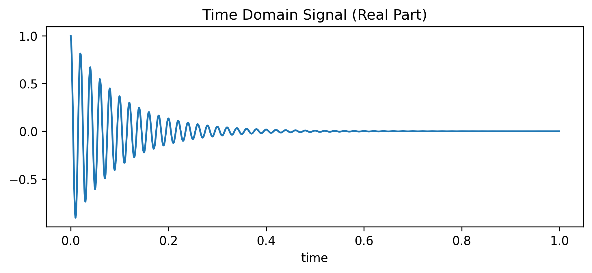
Now, we apply the Fourier transform.
Crucial detail: Because this specific signal starts exactly at , we cannot use the centered wrapper fftc. Applying an ifftshift to the input would physically split our data point and move it to the center of the array, completely destroying the signal phase.
Instead, we use the pure .xmr.fft() followed by an explicit .xmr.fftshift(). By providing out_dim="frequency", the toolbox automatically calculates the reciprocal coordinate values (Hz) based on the input dwell time and renames the dimension for us.
# Transform to Frequency Domain, calculate Hz axis, and center the output
da_spectrum = (
    da_fid
    .xmr.fft(dim="time", out_dim="frequency")
    .xmr.fftshift(dim="frequency")
)

# Plot the real part of the spectrum
fig, ax = plt.subplots(figsize=(8, 3))
da_spectrum.real.plot(ax=ax)
ax.set_title("Frequency Domain Spectrum (Real Part)")
plt.show()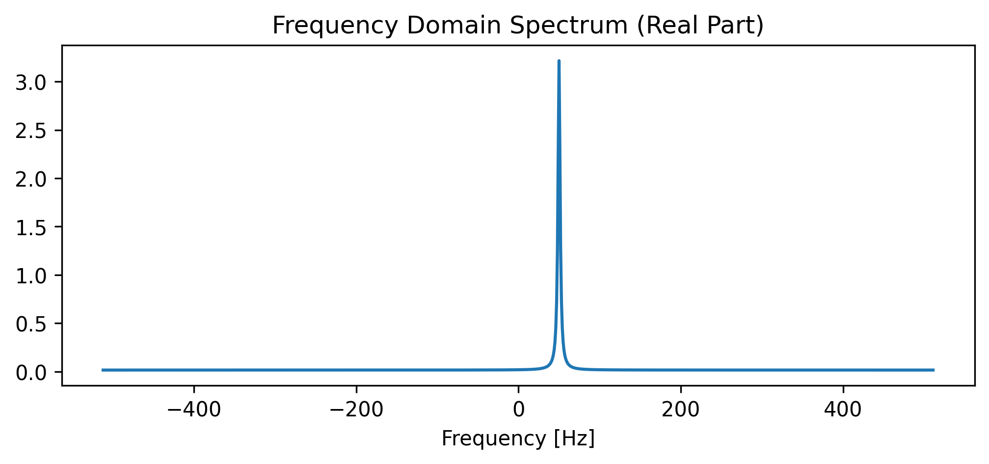
Notebook Cell
# --- AUTOMATED TESTS (Pytest-nbmake) ---
# This cell is hidden in the MyST docs but executed in CI.

# 1. Metadata Preservation & Coordinate Transformation
assert "frequency" in da_spectrum.dims, "Dimension was not renamed!"
assert "time" not in da_spectrum.dims
assert da_spectrum.coords["frequency"].attrs.get("units") == "Hz", "Units were not injected!"

# 2. Check the Math (Is the peak actually at 50 Hz?)
peak_idx = np.argmax(np.abs(da_spectrum.values))
peak_freq = da_spectrum.coords["frequency"].values[peak_idx]
assert np.isclose(peak_freq, 50.0), f"Peak is at {peak_freq} Hz, expected 50 Hz!"

# 3. Parseval's Theorem (Energy Conservation via Ortho Normalization)
energy_time = np.sum(np.abs(da_fid.values) ** 2)
energy_freq = np.sum(np.abs(da_spectrum.values) ** 2)
assert np.isclose(energy_time, energy_freq), "FFT energy conservation failed!"
2. Imaging: 2D -space to Image Space
The true power of xarray + xmris shines in multi-dimensional data. Let’s create a synthetic 2D -space using custom dimension strings ("kx" and "ky"). We will use a simple 2D rectangle, which analytically transforms into a 2D sinc function in the image domain.
# Create a synthetic 2D k-space (64x64 matrix)
kspace_data = np.zeros((64, 64), dtype=complex)
kspace_data[24:40, 24:40] = 1.0  # 16x16 rect in the center

da_kspace = xr.DataArray(
    kspace_data,
    dims=["kx", "ky"],
    coords={"kx": np.linspace(-32, 31, 64), "ky": np.linspace(-32, 31, 64)},
)

# Plot k-space magnitude
fig, ax = plt.subplots(figsize=(5, 5))
ax.imshow(np.abs(da_kspace.values), cmap="gray", extent=[-32, 31, -32, 31])
ax.set_title("k-space (2D Rect)")
plt.show()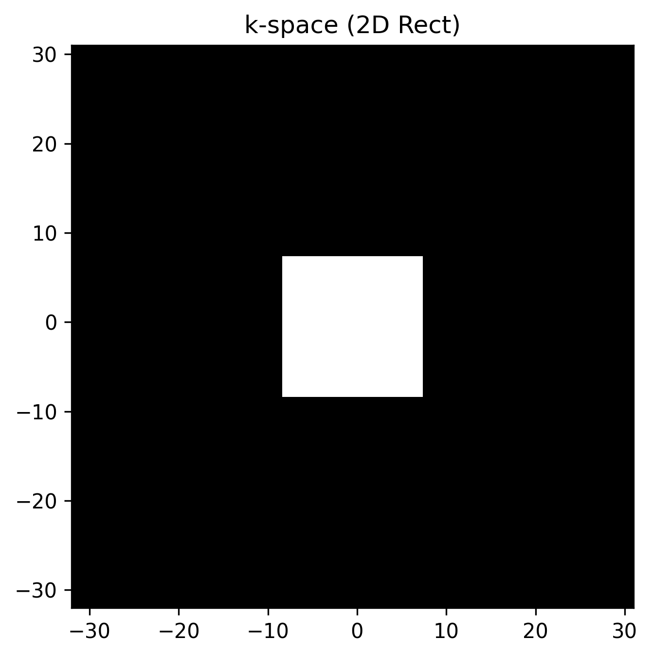
Unlike the 1D signal starting at , imaging data is symmetrically sampled around the center of -space. To transform this correctly, we must shift the input before the transform, and shift the output after.
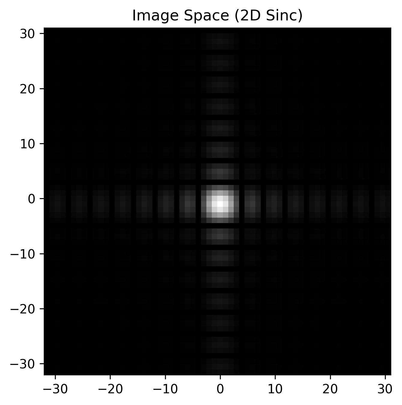
We use the convenience wrapper .xmr.ifftc() to handle these shifts automatically. By passing a list of dimensions, we perform a 2D inverse Fourier transform and seamlessly map ["kx", "ky"] to ["x", "y"] in a single line.
# Transform to Image Domain (2D IFFT with symmetric shifts) and rename dimensions
da_image = da_kspace.xmr.ifftc(dim=["kx", "ky"], out_dim=["x", "y"])

# Plot image domain magnitude
fig, ax = plt.subplots(figsize=(5, 5))
ax.imshow(np.abs(da_image.values), cmap="gray", extent=[-32, 31, -32, 31])
ax.set_title("Image Space (2D Sinc)")
plt.show()