Complex Number Handling

Handling Complex MRI/MRS Data¶

Magnetic resonance data is inherently complex-valued, but many standard tools lack native support for complex numbers. Splitting this data into separate real and imaginary channels is frequently required for:

Machine Learning:
Routing data through standard PyTorch or TensorFlow architectures.
Serialization:
Saving xarray datasets to disk, e.g. da.to_netcdf() and xr.open_dataset().
Visualization:
Plotting real and imaginary components independently.

The xmris accessor provides dedicated utilities (to_real_imag and to_complex) to safely reshape and reconstruct complex xarray.DataArray objects while preserving all metadata and physical coordinates.

import matplotlib.pyplot as plt
import numpy as np
import xarray as xr

# Ensure the accessor is registered
import xmris

1. Splitting Complex Data into Channels¶

Let’s generate a synthetic complex Free Induction Decay (FID) signal.

# Generate a synthetic complex FID
t = np.linspace(0, 1, 512)
complex_fid = np.exp(-t * 3.0) * np.exp(1j * 2 * np.pi * 15.0 * t)

da_complex = xr.DataArray(
    complex_fid,
    dims=["time"],
    coords={"time": t},
    attrs={"B0": 3.0},
    name="Signal",
)

print("Original Shape:", da_complex.shape)
print("Original Dtype:", da_complex.dtype)

Original Shape: (512,)
Original Dtype: complex128

By calling .xmr.to_real_imag(), the array is expanded with a new dimension containing the real and imaginary components.

da_split = da_complex.xmr.to_real_imag()

print("\nSplit Shape:", da_split.shape)
print("Split Dtype:", da_split.dtype)
da_split


Split Shape: (512, 2)
Split Dtype: float64

The array cleanly expanded from (512,) to (512, 2). Because it remains a standard xarray.DataArray, we can easily plot the two channels side-by-side.

fig, ax = plt.subplots(figsize=(8, 4))
da_split.plot.line(ax=ax, x="time", hue="component")
ax.set_title("FID Split into Real and Imaginary Components")
plt.show()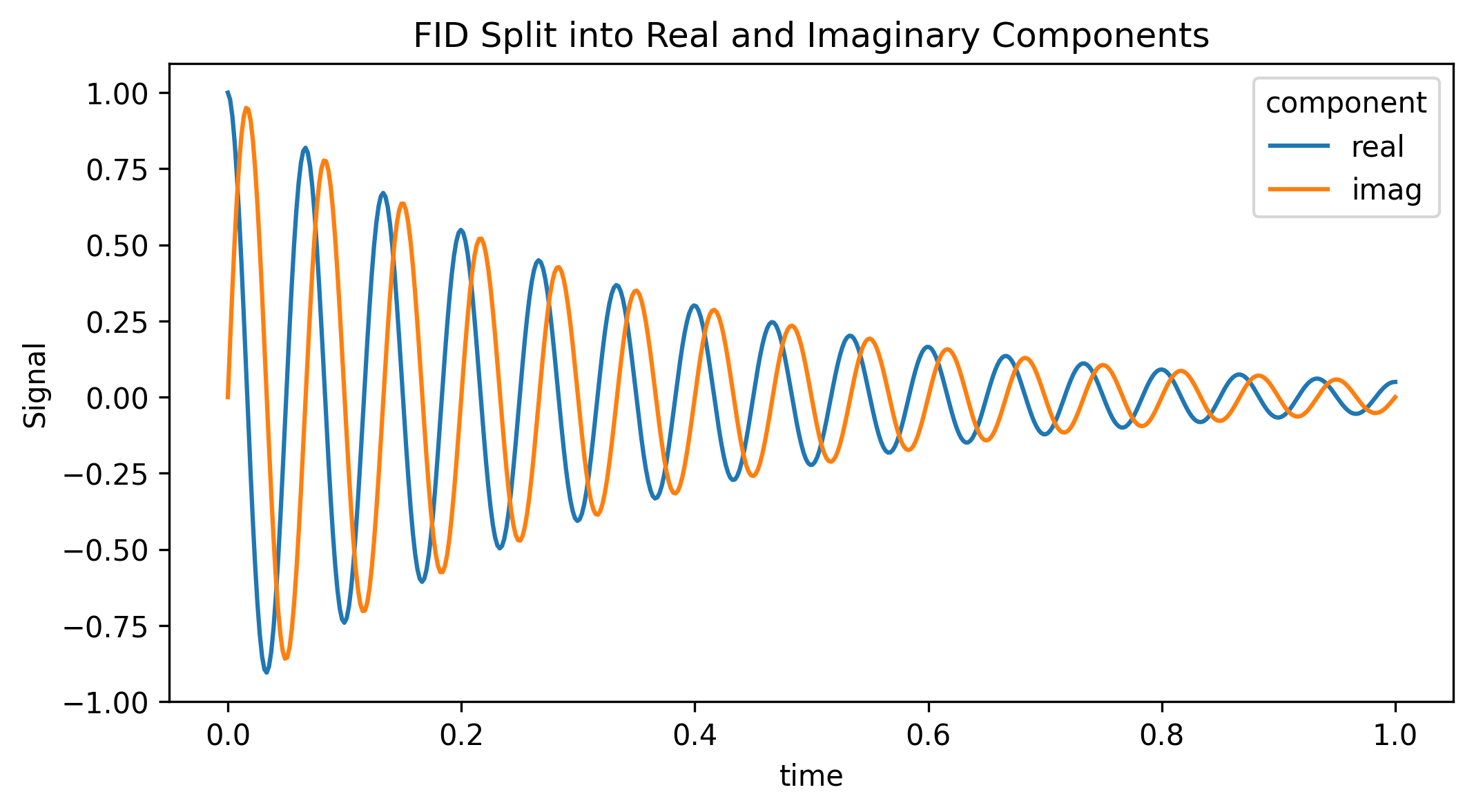

2. Customizing the Split Dimension¶

If your specific ML pipeline expects the channel dimension to have a specific name (e.g., "channel" instead of "component"), you can pass these arguments directly to the function.

da_torch = da_complex.xmr.to_real_imag(dim="channel", coords=("ch0", "ch1"))
print("Custom Dimension:", da_torch.dims)

Custom Dimension: ('time', 'channel')

3. Reconstructing the Complex Array¶

After processing the split channels (e.g., passing them through a neural network), you can seamlessly collapse the dimension back down to a standard complex array for downstream signal processing (like an FFT) using .xmr.to_complex().

da_recon = da_split.xmr.to_complex()

is_identical = np.allclose(da_complex.values, da_recon.values)
print(f"Shape Restored: {da_recon.shape}")
print(f"Data Type Restored: {da_recon.dtype}")
print(f"Exact Mathematical Recovery: {is_identical}")

Shape Restored: (512,)
Data Type Restored: complex128
Exact Mathematical Recovery: True

# STRICT TESTS FOR CI
assert da_split.ndim == da_complex.ndim + 1, "Dimension was not added."
assert da_split.sizes["component"] == 2, "Component dimension should have size 2."
assert not np.iscomplexobj(da_split.values), "Split array should be strictly real."
assert list(da_split.coords["component"].values) == ["real", "imag"]

assert da_recon.ndim == da_complex.ndim, "Reconstruction failed to drop dimension."
assert np.iscomplexobj(da_recon.values), "Reconstructed array should be complex."
assert "component" not in da_recon.dims, "Component dimension was not fully dropped."
np.testing.assert_array_equal(da_recon.values, da_complex.values)
assert da_recon.attrs["B0"] == 3.0, "Reconstruction lost attributes."