Domain Contracts in Action

import matplotlib.pyplot as plt
import matplotlib_inline.backend_inline

# Crisp retina output + sane default DPI for the rendered docs
matplotlib_inline.backend_inline.set_matplotlib_formats("retina")
plt.rcParams["figure.dpi"] = 150

Every xmris operation makes a contract about what you get back: the output domain is a pure function of the operation and the input domain — never a surprise. This page proves the two contracts executable-style; the design story lives in The Two Domains.

You call	on a FID (`time`)	on a spectrum (`frequency`/`chemical_shift`)
`apodize_exp()`, `zero_fill()`	FID ✅	spectrum ✅ (round trip inside)
`autophase()`, `baseline_als()`	spectrum (funnel ⤵)	spectrum
`to_spectrum()`, `to_fid()`	explicit conversion	explicit conversion

Domain-preserving ops compute in the time domain but hand back what you gave them — same physics either side.
Funnel ops are only meaningful on a spectrum, so their result lands there, whatever you feed them.

import numpy as np
import matplotlib.pyplot as plt
import xarray as xr

import xmris  # noqa: F401  (registers the .xmr accessor)
from xmris.fitting.simulation import simulate_fid

1. A distorted, time-domain FID¶

fid = simulate_fid(
    amplitudes=[100, 70, 45],
    chemical_shifts=[2.0, 3.5, 5.0],
    reference_frequency=123.2,
    carrier_ppm=3.0,
    dampings=[25, 25, 30],
    phases=np.deg2rad(65),   # zero-order phase error, baked into the FID
    target_snr=250,
    n_points=2048,
)
fid.dims   # -> ('time',)

('time',)

2. Domain-preserving: same physics, either side¶

Multiplying an FID by $e^{-\pi\,\mathrm{lb}\,t}$ is convolving its spectrum with a Lorentzian of width $\mathrm{lb}$ Hz — one operation, two views. So apodize_exp never changes your representation:

spectrum = fid.xmr.to_spectrum()

fid_smooth = fid.xmr.apodize_exp(lb=3)         # FID in      -> FID out
spec_smooth = spectrum.xmr.apodize_exp(lb=3)   # spectrum in -> spectrum out

print("FID path      :", fid.dims, "->", fid_smooth.dims)
print("spectrum path :", spectrum.dims, "->", spec_smooth.dims)

FID path      : ('time',) -> ('time',)
spectrum path : ('frequency',) -> ('frequency',)

And the two paths are numerically the same operation — transforming the apodized FID reproduces the apodized spectrum to machine precision:

fig, ax = plt.subplots(figsize=(7, 3))
ax.plot(spec_smooth["frequency"], np.real(spec_smooth), lw=2.5, label="spectrum path")
ax.plot(
    spec_smooth["frequency"],
    np.real(fid_smooth.xmr.to_spectrum()),
    lw=1.0,
    ls="--",
    label="FID path → to_spectrum()",
)
ax.set_xlabel("Frequency (Hz)")
ax.set_ylabel("Re{S}")
ax.legend()
ax.grid(True, alpha=0.3)
ax.set_title("Two entry domains, one operation")
plt.tight_layout()
plt.show()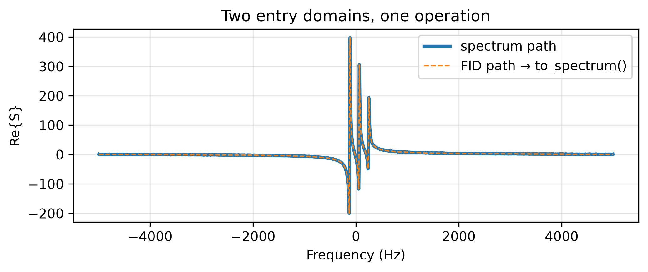

# STRICT TESTS: apodize_exp domain-preserving contract
from xmris.core.config import ATTRS, DIMS

# (a) Representation preserved on both paths.
assert list(fid_smooth.dims) == [DIMS.time]
assert list(spec_smooth.dims) == [DIMS.frequency]

# (b) The two paths are the same operation (unitary round trip, ~1e-12).
np.testing.assert_allclose(
    spec_smooth.values,
    fid_smooth.xmr.to_spectrum().values,
    rtol=1e-10,
    atol=1e-10 * float(np.abs(spec_smooth).max()),
    err_msg="spectrum-path and FID-path apodization must be numerically identical",
)

# (c) Coordinates restored verbatim on the round-tripped path.
np.testing.assert_array_equal(
    spec_smooth.coords[DIMS.frequency].values,
    spectrum.coords[DIMS.frequency].values,
    err_msg="round trip must reassign the original frequency coordinates verbatim",
)

# (d) Attrs survived and the lineage parameter was stamped on both paths.
assert spec_smooth.attrs[ATTRS.apodization_lb] == 3
assert fid_smooth.attrs[ATTRS.apodization_lb] == 3
assert spec_smooth.attrs[ATTRS.reference_frequency] == 123.2

The same contract holds for zero_fill: zero-padding the FID is interpolating the spectrum onto a finer grid — so calling it on a spectrum hands back a spectrum with more points, not a FID:

spec_fine = spectrum.xmr.zero_fill(target_points=4096)
print(spectrum.sizes, "->", spec_fine.sizes)

Frozen({'frequency': 2048}) -> Frozen({'frequency': 4096})

# STRICT TESTS: zero_fill on a spectrum (length-changing round trip)
assert list(spec_fine.dims) == [DIMS.frequency]
assert spec_fine.sizes[DIMS.frequency] == 4096
_freqs = spec_fine.coords[DIMS.frequency].values
assert np.all(np.diff(_freqs) > 0), "recomputed frequency axis must be monotonic"
assert spec_fine.attrs[ATTRS.reference_frequency] == 123.2

3. Funnel: the canonical pipeline, one FFT¶

Phasing and baseline correction exist for the spectrum — their results land there. That makes the classic monotonic pipeline read naturally, with exactly one Fourier transform executing at the funnel boundary:

result = (
    fid.xmr.zero_fill(target_points=4096)   # time-domain home: no transform
       .xmr.apodize_exp(lb=3)               # time-domain home: no transform
       .xmr.autophase()                     # funnel: FID -> spectrum, stays
       .xmr.baseline_als()                  # already spectral: no transform
)
print("pipeline result:", result.dims, "| real-valued:", not np.iscomplexobj(result.values))

pipeline result: ('frequency',) | real-valued: True

ppm = result.xmr.to_ppm()
fig, ax = plt.subplots(figsize=(7, 3))
ax.plot(ppm["chemical_shift"], ppm.values, lw=1.5)
ax.axhline(0, color="red", ls="--", alpha=0.4)
ax.set_xlabel("Chemical shift (ppm)")
ax.set_ylabel("Re{S}")
ax.invert_xaxis()
ax.grid(True, alpha=0.3)
ax.set_title("zero_fill → apodize → autophase → baseline, straight from the FID")
plt.tight_layout()
plt.show()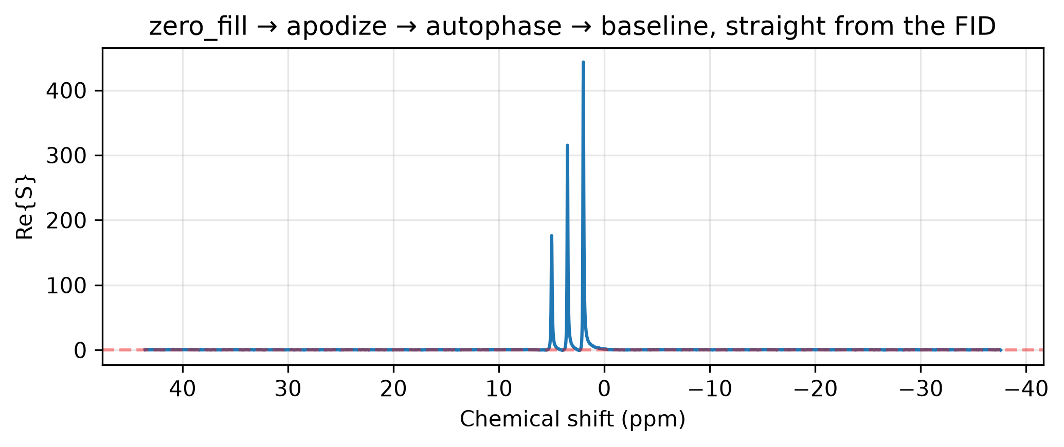

# STRICT TESTS: the canonical pipeline
# (a) Landed in the spectral domain (funnel), real-valued after baseline.
assert DIMS.frequency in result.dims
assert DIMS.time not in result.dims
assert not np.iscomplexobj(result.values)
assert result.sizes[DIMS.frequency] == 4096

# (b) The full lineage of quantitative parameters was recorded.
assert result.attrs[ATTRS.apodization_lb] == 3
assert ATTRS.phase_p0 in result.attrs
assert ATTRS.phase_p1 in result.attrs

# (c) Physics metadata survived the whole chain (issue #21 guarantee).
assert result.attrs[ATTRS.reference_frequency] == 123.2
assert result.attrs[ATTRS.carrier_ppm] == 3.0

4. Guardrails¶

One-way data fails loudly. baseline_als discards the imaginary component, so no valid FID exists behind its output — a time-domain op on it refuses rather than inventing one:

try:
    result.xmr.apodize_exp(lb=2)
except ValueError as err:
    print(err)

Cannot transform real-valued spectral data (dim 'frequency') into the time domain: the imaginary component is gone (e.g. discarded by `baseline_als`), so no valid FID exists behind this spectrum.

Apply time-domain operations before the step that discarded the imaginary part, or pass an explicit existing dimension to operate on.

Explicit foreign dims pass through — for domain-preserving ops. A domain-preserving op named on an axis outside its domain skips conversion entirely — naming another axis (k-space, say) leaves the data untouched. (Funnel ops have no passthrough: they always land in their home domain.)

rng = np.random.default_rng(42)
kspace = xr.DataArray(
    rng.standard_normal((8, 8)),
    dims=["kx", "ky"],
    coords={"kx": np.arange(8), "ky": np.arange(8)},
)
kfilled = kspace.xmr.zero_fill(dim="kx", target_points=16, position="symmetric")
print(dict(kspace.sizes), "->", dict(kfilled.sizes))

{'kx': 8, 'ky': 8} -> {'kx': 16, 'ky': 8}

# STRICT TESTS: guardrails
# (a) Complexity gate: real-valued spectral data cannot go to the time domain.
_raised = False
try:
    result.xmr.apodize_exp(lb=2)
except ValueError as _err:
    _raised = True
    assert "real-valued" in str(_err)
assert _raised, "the complexity gate must reject real-valued spectral input"

# (b) Passthrough: explicit foreign dim disables coercion entirely.
assert list(kfilled.dims) == ["kx", "ky"]
assert kfilled.sizes["kx"] == 16 and kfilled.sizes["ky"] == 8