Domain-Agnostic Autophase

import matplotlib.pyplot as plt
import matplotlib_inline.backend_inline

# Crisp retina text + sane default DPI for the rendered docs
matplotlib_inline.backend_inline.set_matplotlib_formats("retina")
plt.rcParams["figure.dpi"] = 100

Phase correction is a frequency-domain operation, but the data you have in hand is often a time-domain FID. Classically that forces you to remember the ritual:

spectrum = fid.xmr.to_spectrum().xmr.autophase()   # you must FFT first, by hand

autophase now removes that ceremony — hand it a FID and it Fourier-transforms into the frequency domain for you, then phases:

spectrum = fid.xmr.autophase()   # auto-FFT happens under the hood

This is powered by the domain-contract taxonomy: a gate decorator plus two domain decorators sharing one engine, each declaring a function’s contract at the definition site.

Tier	Decorator	Contract	Cost
gate	`@requires_attrs(...)`	raises if metadata is missing	$O(1)$
domain — funnel	`@ensures_domain(...)`	transforms into the home domain, result stays there	$O(N \log N)$
domain — preserving	`@computes_in(...)`	round-trips through the home domain, representation restored	$O(N \log N)$

Both domain decorators also resolve the working axis: a dim=None argument is filled with the spectral dimension actually present (frequency [Hz] or chemical_shift [ppm]) — an explicit dim is never overridden.

autophase is a funnel operation — you phase in order to inspect the spectrum, so the result lands there:

A FID $s(t)$ and its spectrum $S(\nu)$ are a Fourier pair, $S(\nu) = \mathcal{F}\{s(t)\}$ , and phase correction acts on the spectrum,

S_\text{phased}(\nu) = S(\nu)\, \exp\!\left[i\left(p_0 + p_1\,\frac{\nu - \nu_\text{pivot}}{\Delta\nu}\right)\right].

(1)

@ensures_domain supplies the $\mathcal{F}$ so you can start from either side.

import numpy as np
import matplotlib.pyplot as plt

import xmris  # registers the .xmr accessor
from xmris.fitting.simulation import simulate_fid


def plot_real(spectra, title):
    """Plot the real part of one or more spectra against the ppm axis."""
    fig, axes = plt.subplots(len(spectra), 1, figsize=(7, 2.4 * len(spectra)), sharex=True)
    axes = np.atleast_1d(axes)
    for ax, (da, label) in zip(axes, spectra):
        ppm = da.xmr.to_ppm()
        ax.plot(ppm.coords["chemical_shift"], np.real(ppm.values), lw=1.5)
        ax.axhline(0, color="red", ls="--", alpha=0.4)
        ax.set_ylabel("Re{S}")
        ax.legend([label], loc="upper right")
        ax.grid(True, alpha=0.3)
    axes[-1].set_xlabel("Chemical shift (ppm)")
    axes[-1].invert_xaxis()
    fig.suptitle(title)
    plt.tight_layout()
    plt.show()

Hand it a raw FID¶

We simulate a noisy, time-domain FID with a 65° zero-order phase error baked in. Note the dimension: this is a FID, not a spectrum.

fid = simulate_fid(
    amplitudes=[100, 70, 45],
    chemical_shifts=[2.0, 3.5, 5.0],
    reference_frequency=123.2,
    carrier_ppm=3.0,
    dampings=[25, 25, 30],
    phases=np.deg2rad(65),   # zero-order phase distortion, baked into the FID
    target_snr=250,
    n_points=2048,
)
fid.dims   # -> ('time',)

('time',)

Now call autophase directly on the FID. There is no to_spectrum() in the chain — @ensures_domain performs the FFT, and the output comes back as a spectrum.

raw_spectrum = fid.xmr.to_spectrum()   # for comparison: the distorted spectrum
phased = fid.xmr.autophase()           # auto-FFT + autophase, straight from the FID

print("input FID :", fid.dims)
print("phased    :", phased.dims, "| p0 = %.1f°, p1 = %.1f°"
      % (phased.attrs["phase_p0"], phased.attrs["phase_p1"]))

input FID : ('time',)
phased    : ('frequency',) | p0 = -60.2°, p1 = 107.2°

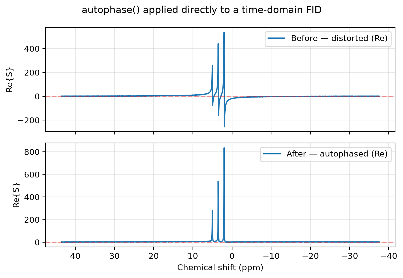
The distorted spectrum has its signal smeared between the real (absorptive) and imaginary (dispersive) channels; after autophasing the peaks stand up cleanly in the real part.

plot_real(
    [(raw_spectrum, "Before — distorted (Re)"), (phased, "After — autophased (Re)")],
    "autophase() applied directly to a time-domain FID",
)

from xmris.core.config import ATTRS, DIMS

# 1. The auto-FFT ran: output is a spectrum, and the time axis is gone.
assert DIMS.frequency in phased.dims
assert DIMS.time not in phased.dims

# 2. Metadata survived the auto-FFT (the issue #21 guarantee).
assert phased.attrs[ATTRS.reference_frequency] == 123.2
assert phased.attrs[ATTRS.carrier_ppm] == 3.0

# 3. Phase lineage was recorded.
assert ATTRS.phase_p0 in phased.attrs
assert ATTRS.phase_p1 in phased.attrs

# 4. Correctness: phasing concentrates signal into the real (absorptive) part,
#    so the real-valued peak is taller than in the distorted spectrum.
assert np.real(phased).max() > np.real(raw_spectrum).max()

Already a spectrum? No extra FFT.¶

The same call on data that is already spectral is a no-op on the domain — the ensures tier sees a spectral dimension and passes the array straight through, so nothing is transformed twice.

spectrum = fid.xmr.to_spectrum()   # already frequency-domain
phased_again = spectrum.xmr.autophase()

print("input :", spectrum.dims, "-> output:", phased_again.dims)   # frequency in, frequency out

input : ('frequency',) -> output: ('frequency',)

Whether you start from the FID or the spectrum, autophase does the right thing — the domain plumbing is handled for you, and the output honestly reports where it landed.