title: Spectrum - Phase Correction¶

import matplotlib.pyplot as plt
import matplotlib_inline.backend_inline

# 1. Use retina for crisp, PDF-like text that never disappears in HTML
matplotlib_inline.backend_inline.set_matplotlib_formats("retina")

# 2. Set a high baseline DPI
plt.rcParams["figure.dpi"] = 150

Phase correction is a crucial frequency-domain operation applied after the Fourier Transform. Due to hardware delays, filter group delays, and off-resonance effects, the real part of the resulting complex spectrum often contains a mixture of absorptive and dispersive lineshapes, rather than pure absorptive peaks.

A phase correction applies a frequency-dependent phase angle, $\phi(\omega)$, to the spectrum:

Where the phase angle is modeled as a linear polynomial consisting of a zero-order (frequency-independent) term $p_0$ and a first-order (frequency-dependent) term $p_1$. To ensure the first-order twist scales predictably regardless of the spectral sweep width, $p_1$ is anchored around a physical pivot coordinate (by default, the point of maximum magnitude) and scaled by the absolute spectral range:

import matplotlib.pyplot as plt
import numpy as np
import xarray as xr

# Ensure the accessor is registered
import xmris

1. Generating Synthetic Unphased Data¶

Let’s generate a synthetic, noisy Free Induction Decay (FID) with two distinct peaks, convert it to a spectrum, and then intentionally apply severe zero- and first-order phase errors to simulate raw scanner data.

Source

# Acquisition parameters
dwell_time = 0.001  # 1 ms
n_points = 1024
t = np.arange(n_points) * dwell_time

# Synthetic FID: Two peaks at 50 Hz and -150 Hz
rng = np.random.default_rng(42)
clean_fid = np.exp(-t / 0.05) * (
    np.exp(1j * 2 * np.pi * 50 * t) + 0.6 * np.exp(1j * 2 * np.pi * -150 * t)
)
noise = rng.normal(scale=0.08, size=n_points) + 1j * rng.normal(scale=0.08, size=n_points)
raw_fid = clean_fid + noise

# Xarray construction and FFT
da_fid = xr.DataArray(
    raw_fid, dims=["time"], coords={"time": t}, attrs={"sequence": "sLASER", "B0": 7.0}
)
da_spec = da_fid.xmr.to_spectrum()

# Intentionally ruin the phase: p0 = 120 degrees, p1 = -45 degrees
# The pivot defaults to the peak with the maximum magnitude (50 Hz)
da_ruined = da_spec.xmr.phase(p0=120.0, p1=-45.0)

fig, axes = plt.subplots(1, 2, figsize=(12, 3))
da_spec.real.plot(ax=axes[0], color="tab:blue")
axes[0].set_title("Target 'Clean' Spectrum (Real Part)")

da_ruined.real.plot(ax=axes[1], color="tab:red")
axes[1].set_title("Unphased Spectrum (Real Part)")
plt.tight_layout()
plt.show()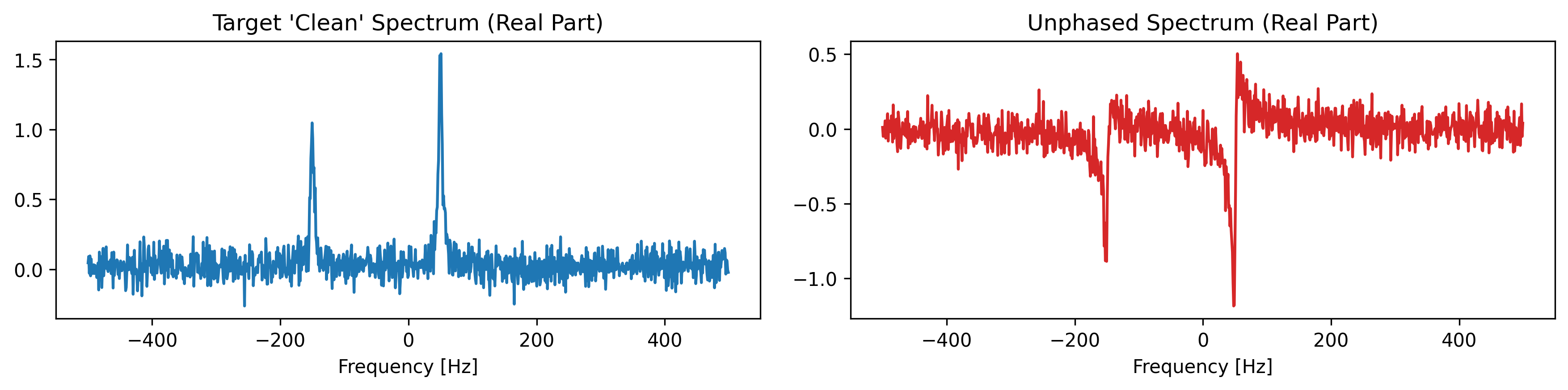

2. Manual Phase Correction¶

We can manually apply zero- and first-order phase correction (in degrees) using the .xmr.phase() method. Because this is an xarray accessor, the exact quantifiable phase angles used are permanently appended to the DataArray attributes (as phase_p0, phase_p1, and phase_pivot) to safely preserve the data lineage.

Since we know we ruined the spectrum with $p_0 = 120^\circ$ and $p_1 = -45^\circ$, we can restore it by applying the exact inverse. Because phase corrections do not alter the absolute magnitude of the spectrum, the default calculated pivot remains perfectly symmetric!

# Apply the inverse phase angles and specify the dimension
da_manual = da_ruined.xmr.phase(dim="frequency", p0=-120.0, p1=45.0)

fig, ax = plt.subplots(figsize=(8, 3))
da_ruined.real.plot(ax=ax, color="lightgray", label="Unphased")
da_manual.real.plot(ax=ax, color="tab:blue", label="Manually Phased")
plt.legend()
plt.title("Manual Phase Correction")
plt.show()

# Print the attributes to see the strictly tracked mathematical lineage
print("Stored Phase Attributes:")
print(f"  phase_p0: {da_manual.attrs.get('phase_p0')}")
print(f"  phase_p1: {da_manual.attrs.get('phase_p1')}")
print(f"  phase_pivot: {da_manual.attrs.get('phase_pivot')}")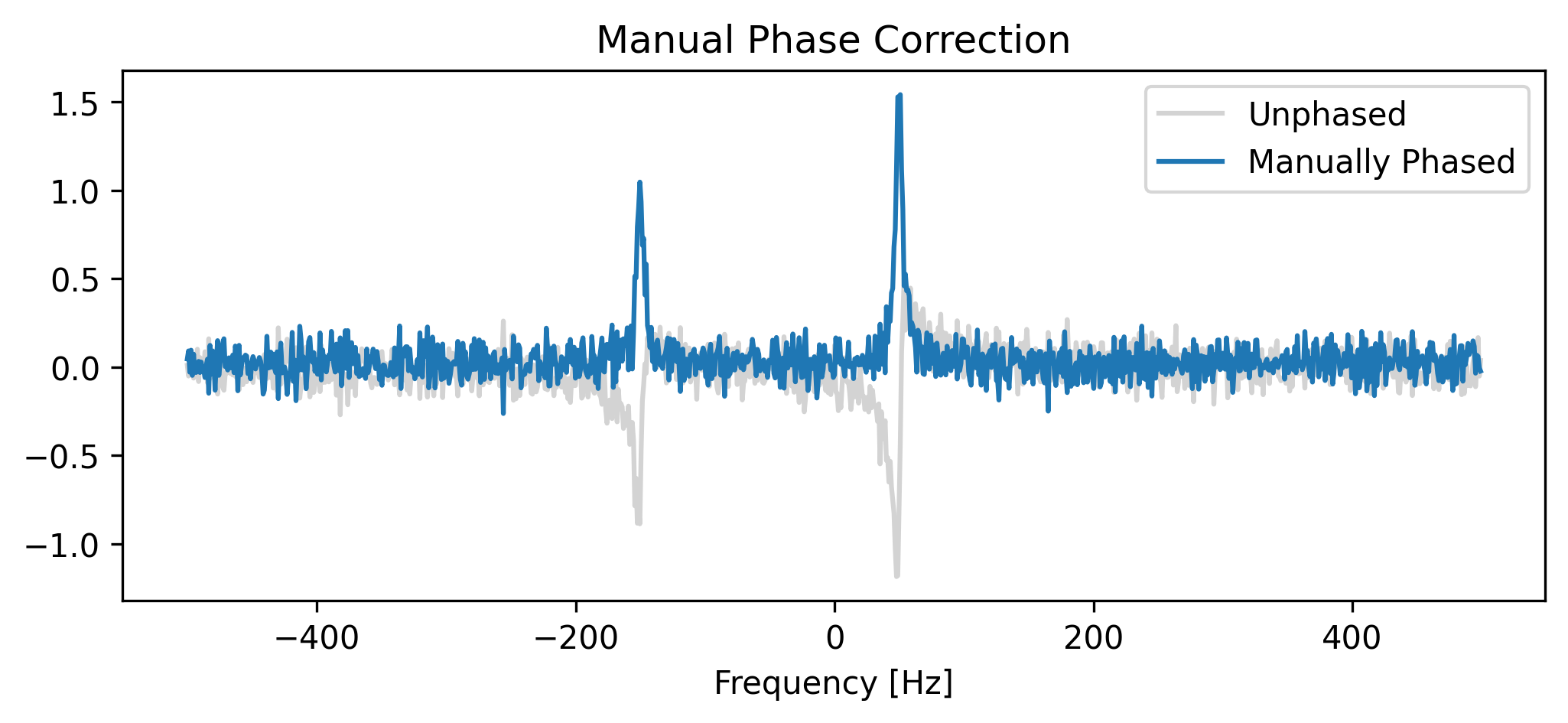

Stored Phase Attributes:
  phase_p0: -120.0
  phase_p1: 45.0
  phase_pivot: 48.828125

# STRICT TESTS: Manual Phase Correction
assert "phase_p0" in da_manual.attrs and "phase_p1" in da_manual.attrs
assert "phase_pivot" in da_manual.attrs
assert da_manual.attrs["phase_p0"] == -120.0
assert da_manual.attrs["phase_p1"] == 45.0

# Prove metadata preservation
assert da_manual.dims == da_ruined.dims, "Dimensions altered."
np.testing.assert_array_equal(
    da_manual.coords["frequency"].values,
    da_ruined.coords["frequency"].values,
    err_msg="Coords altered.",
)
assert da_manual.attrs["sequence"] == "sLASER", "Original attributes dropped."

# Prove exact mathematical recovery (allowing for small floating point drift)
np.testing.assert_allclose(
    da_manual.values,
    da_spec.values,
    rtol=1e-5,
    atol=1e-5,
    err_msg="Manual phase math failed to invert.",
)

Next up: Automated Phase Correction (autophase)¶

Finding the perfect phase angles manually is tedious. We can use algorithms such as entropy-minimization algorithm (ACME) to find the global phase minimum automatically.