A spectrum shows you that a peak is there. Quantitative MRS needs to know how much — an
amplitude per metabolite, with an honest error bar on it. That is what time-domain fitting
delivers, and in xmris it is three steps: get a signal, say which peaks you expect, hand both to
fit_amares.
This page is the shortest path from an FID to a table of numbers. Everything it glosses over — what else is in the returned object, whether you should believe it, what happens across a whole imaging grid — is picked up by AMARES Fitting in Depth.
| Function | What it does here |
|---|---|
simulate_fid() | stands in for the scanner: a synthetic ³¹P FID |
build_prior_knowledge() | turns a dict of named peaks into AMARES prior knowledge |
.xmr.fit_amares() | fits the signal and returns a Dataset |
.xmr.to_spectrum() | FID → spectrum, for looking at it |
.xmr.to_ppm() | relabels the frequency axis in ppm |
import numpy as np

import xmris  # registers the .xmr accessor
from xmris import build_prior_knowledge
from xmris.fitting.simulation import simulate_fid
1. A spectrum to fit
Real data would come off a scanner — the Bruker loader hands you the same kind of array. Here we simulate a ³¹P FID at 7 T: phosphocreatine (PCr) at 0 ppm and γ-ATP at −7.5 ppm, with a realistic noise floor.
fid = simulate_fid(
    amplitudes=[10.0, 5.0],                    # PCr twice the size of γ-ATP
    chemical_shifts=[0.0, -7.5],               # ppm
    reference_frequency=120.6,                 # MHz — 31P at 7 T
    spectral_width=8000.0,                     # Hz
    n_points=512,
    dampings=[np.pi * 15.0, np.pi * 20.0],     # damping = pi * linewidth [Hz]
    target_snr=60.0,
    seed=0,                                    # reproducible noise
)

fid.xmr.to_spectrum().xmr.to_ppm().real.plot(figsize=(7, 3))
plt.gca().invert_xaxis()  # NMR convention: ppm decreases to the right
plt.show()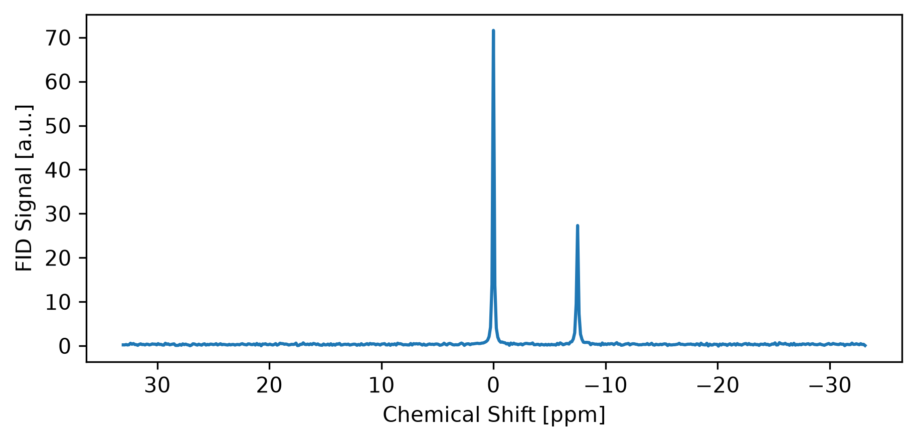
2. Say what you expect to find
AMARES does not search for peaks — you tell it what is there, and it refines your description until the model matches the signal. That description is the prior knowledge: a starting value and a range for every peak’s amplitude, chemical shift, linewidth and phase.
build_prior_knowledge takes named peaks and plain numbers. Only amplitude, chem_shift and
linewidth are required; phase, lineshape and the bounds fall back to safe defaults.
pk = {
    "PCr": {"amplitude": 10.0, "chem_shift": 0.0, "linewidth": 15.0},
    "ATP": {"amplitude": 5.0, "chem_shift": -7.5, "linewidth": 20.0},
}
Your starting numbers do not have to be right — they have to be close. Each shift gets a ±0.5 ppm search window around the value you gave, and each amplitude is free to move upward from it.
What that dict becomes
pyAMARES reads prior knowledge from a positional CSV: an Initial Values block, then a Bounds
block, peaks as columns. Easy to read, fiddly to write by hand — which is the point of the builder.
You never need this file (the dict goes straight into the fit), but it is worth seeing once:
Index,PCr,ATP
Initial Values,,
amplitude,10.0,5.0
chemicalshift,0.0,-7.5
linewidth,15.0,20.0
phase,0.0,0.0
g,0.0,0.0
Bounds,,
amplitude,"(0.0, ","(0.0, "
chemicalshift,"(-0.5, 0.5)","(-8.0, -7.0)"
linewidth,"(0.0, ","(0.0, "
phase,"(-180.0, 180.0)","(-180.0, 180.0)"
g,"(0.0, 1.0)","(0.0, 1.0)"
3. Fit it
One call. It takes the prior knowledge, fits in the time domain, and returns everything it learned
as an xarray.Dataset.
ds = fid.xmr.fit_amares(pk)
dsExpand the arrays above and you can already see the shape of the answer: data, fit and
residuals still live on time, while amplitude, chem_shift, linewidth, phase and snr
sit on a new metabolite axis carrying your peak names. Uncertainties (crlb, sd) span one more
axis, parameter, so a single variable holds the error on every fitted quantity.
4. Read the numbers
The quantified variables all share the metabolite axis, so they tabulate directly — no NumPy
slicing, no bookkeeping about which row was which peak.
table = ds[["amplitude", "chem_shift", "linewidth", "phase", "snr"]].to_dataframe()
table["crlb_%"] = ds["crlb"].sel(parameter="amplitude").to_series()
table.round(2)crlb_% is the Cramér–Rao lower bound on each amplitude — the smallest uncertainty any unbiased
fit of this data could achieve, as a percentage of the amplitude itself. Under a percent here,
because this signal is clean; on real data it is the number that tells you whether to trust a
value.
Numbers are only half of it. The other half is looking at what the model actually did, which is why the fitted signal and the residual come back alongside the parameters:
spec_data = ds["data"].xmr.to_spectrum().xmr.to_ppm()
spec_fit = ds["fit"].xmr.to_spectrum().xmr.to_ppm()
spec_res = ds["residuals"].xmr.to_spectrum().xmr.to_ppm()

fig, ax = plt.subplots(figsize=(7, 4))
spec_data.real.plot(ax=ax, color="black", alpha=0.4, label="data")
spec_fit.real.plot(ax=ax, color="tab:red", lw=1.5, label="fit")
(spec_res.real - 8).plot(ax=ax, color="tab:green", lw=1, label="residual (offset)")

ax.invert_xaxis()
ax.set_ylabel("intensity [a.u.]")
ax.set_title("Fit quality, voxel by eye")
ax.legend()
plt.show()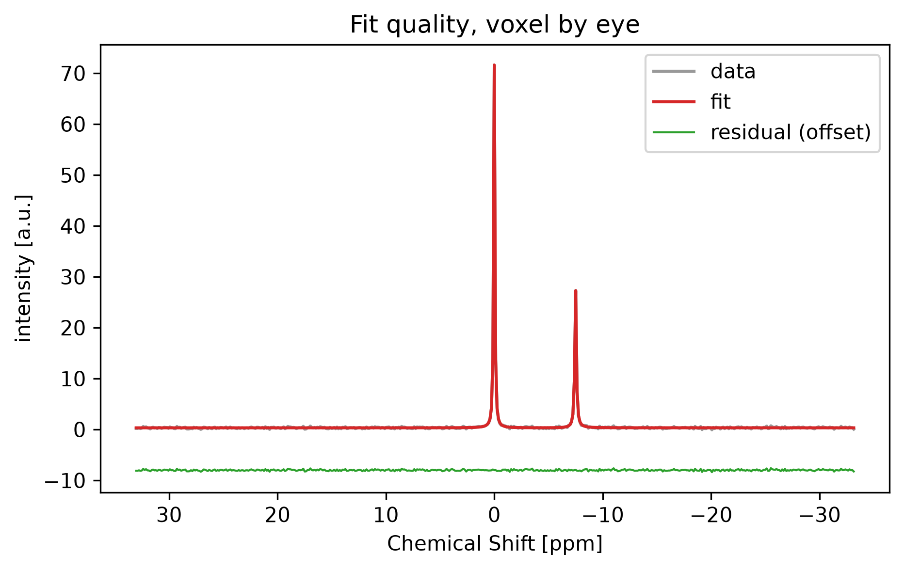
A residual that looks like the noise it was drawn from — flat, structureless, centred on zero — is what a converged fit looks like. Structure left under a peak means the model is missing something.