Fitting one clean spectrum is three lines. Fitting a real dataset raises three questions that page never had to answer: what happens to the other voxels, what is actually inside the object that comes back, and how do you know which of those numbers to believe?
This page answers them on data built to misbehave — peaks that drift, signal that fades, a voxel with nothing in it at all — using the same one-line call throughout.
Why AMARES?
From the pyAMARES paper:
AMARES models the MRS signal as a sum of exponentially damped sinusoids. It uses parameters such as chemical shift, linewidth, amplitude, phase, and spectral lineshape, which can be constrained by prior knowledge. This knowledge includes initial parameters, parameter ranges, and relationships between different peaks and can be readily obtained from published literature. Peaks outside the region of interest can be filtered out, and parameters without prior knowledge can be fitted.
In contrast, frequency-domain fitting methods like LCModel require all metabolites to be modeled as basis set spectra. While this approach reduces the number of parameters to fit, it requires additional effort to obtain basis set spectra through experiments or numerical simulations. Moreover, frequency-domain fitting strategies typically require well-phased absorptive spectra. AMARES circumvents the sometimes subjective and complicated phasing procedure, making it particularly effective for analyzing data with distorted phases due to long receiver dead times.
LCModel and AMARES have been compared directly and proven to be comparable, each with its own advantages. However, AMARES is often the preferred method for quantifying X-nuclei MRS data, such as 13C and 31P MRS, where spectra typically exhibit fewer peaks and less J-coupling compared to 1H MRS.
| Function | What it does here |
|---|---|
simulate_fid() | builds one voxel of synthetic ³¹P signal at a time |
build_prior_knowledge() | validates the peak dict below — fit_amares calls it for you |
.xmr.fit_amares() | fits every voxel in one call, returns a Dataset |
.xmr.to_spectrum() | FID → spectrum, across all voxels at once |
.xmr.to_ppm() | relabels the frequency axis in ppm |
.xmr.to_hz() | and back again |
import numpy as np
import pandas as pd
import xarray as xr

import xmris  # registers the .xmr accessor
from xmris.fitting.simulation import simulate_fid
1. A dataset worth fitting¶
A textbook spectrum is a bad test. Real spectroscopic imaging goes wrong in ways that are boring individually and awkward together: B0 inhomogeneity shifts every peak in a voxel by a fraction of a ppm, coil sensitivity falls off with distance so the noise floor is not the same twice, and some voxels sit outside the object and contain nothing to fit.
So we simulate a row of eight voxels with all three. simulate_fid makes one voxel at a time —
each with its own concentration, its own frequency offset and its own noise level — and xr.concat
stacks them into the 2-D (voxel, time) array that fitting expects.
n_voxels = 8
mhz = 120.6  # 31P at 7 T

pcr_amplitude = np.linspace(10.0, 45.0, n_voxels)   # concentration rises along the row
b0_drift = np.linspace(-0.25, 0.25, n_voxels)       # ppm — the shim degrades across it
snr = np.geomspace(250.0, 4.0, n_voxels)            # coil sensitivity falls off with distance

voxels = [
    simulate_fid(
        amplitudes=[pcr_amplitude[i], 5.0],                    # PCr varies, ATP does not
        chemical_shifts=[0.0 + b0_drift[i], -7.5 + b0_drift[i]],
        reference_frequency=mhz,
        spectral_width=8000.0,
        n_points=512,
        dampings=[np.pi * 15.0, np.pi * 20.0],
        target_snr=float(snr[i]),
        seed=i,  # a different noise draw per voxel, still reproducible
    )
    for i in range(n_voxels)
]

voxels[3] = xr.zeros_like(voxels[3])  # this one is outside the object: no signal at all

grid = xr.concat(voxels, dim="voxel").assign_coords(voxel=np.arange(n_voxels))
grid.attrs = {"reference_frequency": mhz, "carrier_ppm": 0.0}
gridPlotted, the three effects are hard to miss — and hard to fit:
spectra = grid.xmr.to_spectrum().xmr.to_ppm()

fig, axes = plt.subplots(1, 2, figsize=(10, 4))
spectra.real.plot.line(x="chemical_shift", hue="voxel", ax=axes[0], add_legend=False)
axes[0].set_title("The row: PCr grows, noise grows with it")
axes[0].set_xlim(4, -12)

spectra.real.plot.line(x="chemical_shift", hue="voxel", ax=axes[1])
axes[1].set_title("Zoom on PCr: every voxel sits somewhere else")
axes[1].set_xlim(0.6, -0.6)

for ax in axes:
    ax.set_ylabel("intensity [a.u.]")
plt.tight_layout()
plt.show()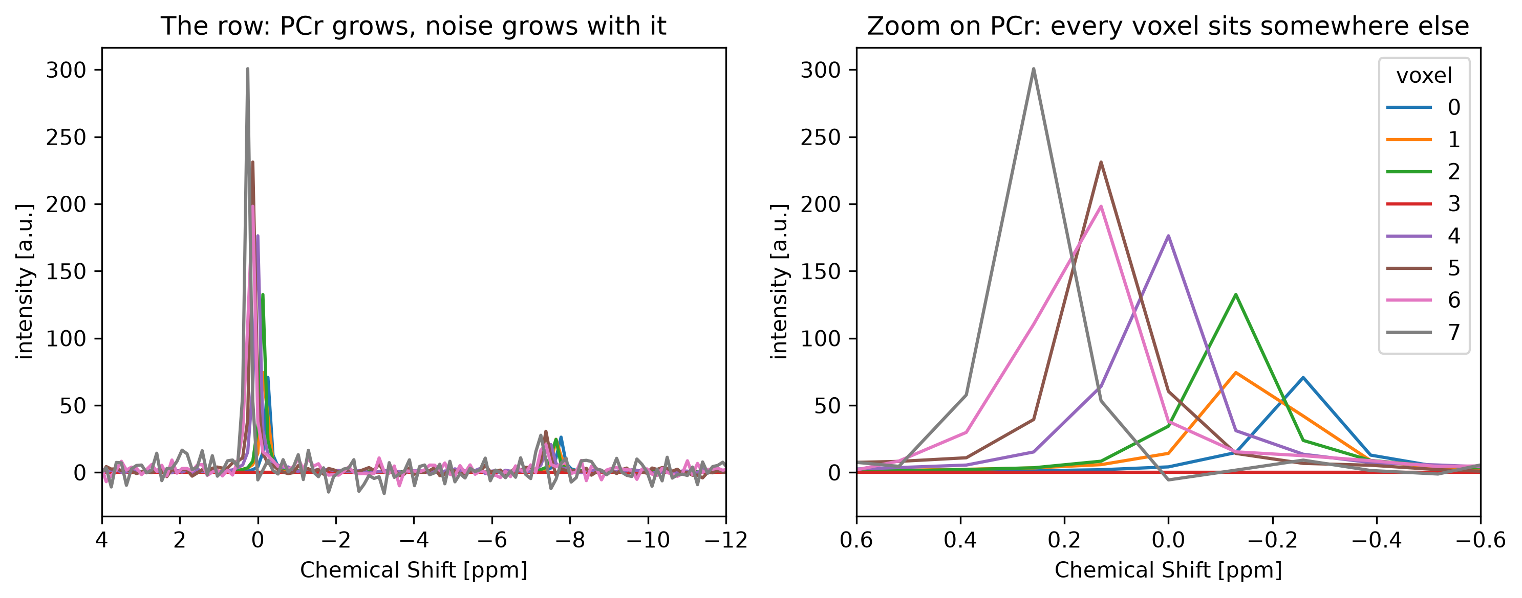
2. One call, every voxel¶
The prior knowledge is the same as for a single spectrum, with one adjustment: the default ±0.5 ppm search window is generous here, but stating the window explicitly documents how much drift you expect the fit to absorb.
pk = {
    "PCr": {
        "amplitude": 10.0,
        "chem_shift": 0.0,
        "linewidth": 15.0,
        "chem_shift_bounds": (-0.6, 0.6),
    },
    "ATP": {
        "amplitude": 5.0,
        "chem_shift": -7.5,
        "linewidth": 20.0,
        "chem_shift_bounds": (-8.2, -6.8),
    },
}
Now the part that would otherwise be a for loop. fit_amares flattens every non-time dimension
into a single list of spectra, scans it for the highest-SNR one to initialize the pyAMARES template
from, fits each in turn, and reassembles the results onto the axes you started with.
ds = grid.xmr.fit_amares(pk)Two arguments worth knowing about, neither of them required:
num_workersdecides whether those fits are spread over worker processes. It defaults to1— everything in-process — because a pool costs a second or two to start, which eight 512-point spectra never earn back. On a real grid the arithmetic reverses: pass-1for every core, or-2to leave one free. The diary entry has the measurements, including the two very different break-even points, and the reason the default stays serial.methodpicks the optimizer, and the default"least_squares"(SciPy’s trust-region solver) is the one to keep."leastsq"— Levenberg–Marquardt — is faster per fit, but on drifted data like this it has a second, shallower minimum it settles into unpredictably, so the same signal fitted twice can give amplitudes 22% apart with both fits reporting success. The diary entry has the measurements.
3. Anatomy of the returned Dataset¶
Fitting is the one xmris operation that does not hand back a DataArray. It cannot: a fit produces
signals that live on time, quantities that live per metabolite, and uncertainties that live per
metabolite and per parameter. Three different shapes, one aligned container.
ds| Shape | Variables | What it is |
|---|---|---|
(voxel, time) | data, fit, residuals | the signal you passed in, the model AMARES built, and what is left over |
(voxel, metabolite) | amplitude, chem_shift, linewidth, phase, snr | the quantified answer, one number per peak per voxel |
(voxel, metabolite, parameter) | crlb, sd | the uncertainty on every fitted parameter, relative (%) and absolute |
(voxel,) | fit_status | whether that voxel was fitted at all |
The point of the metabolite and parameter axes is that they carry names, so selection reads
like the question you are asking:
print("PCr amplitude, all voxels:", ds["amplitude"].sel(metabolite="PCr").values.round(2))
print("its uncertainty (%)      :", ds["crlb"].sel(metabolite="PCr", parameter="amplitude").values.round(2))
print("worst parameter per voxel:", ds["crlb"].max("parameter").sel(metabolite="PCr").values.round(2))
PCr amplitude, all voxels: [10. 15. 20. nan 29.97 34.48 40.58 42.5 ]
its uncertainty (%) : [0.06 0.1 0.19 nan 0.6 1.03 1.94 3.36]
worst parameter per voxel: [ 67.77 98.24 204.15 nan 724.29 87.32 2745.26 230.17]
Lineage survives the fit, and the fit adds its own:
ds.attrs{'reference_frequency': 120.6,
'carrier_ppm': 0.0,
'amares_amplitude_scale': 54.76378690227429}amares_amplitude_scale is the single factor the whole array was divided by before fitting.
pyAMARES derives its optimizer tolerance from signal magnitude, so a Bruker-scale FID would
otherwise “converge” before the solver moved; xmris normalizes once, fits, and multiplies the
amplitudes back. Recording the factor keeps that auditable rather than hidden.
Which voxels were actually fitted¶
Voxel 3 was empty. It could not be fitted, and the honest record of that is not a zero — a zero is a measurement, and a downstream mean would fold it in as though somebody had measured nothing there.
print("amplitude:", ds["amplitude"].sel(metabolite="PCr").values.round(2))
print("fit_status:", ds["fit_status"].values)
print(ds["fit_status"].attrs)
amplitude: [10. 15. 20. nan 29.97 34.48 40.58 42.5 ]
fit_status: [0 0 0 1 0 0 0 0]
{'flag_values': [0, 1, 2], 'flag_meanings': 'fitted no_signal failed'}
NaN says there is no value here. fit_status says why: 0 fitted, 1 no signal to fit,
2 the solver was handed a real spectrum and failed on it. The first two are visible above; the
third is the one worth grepping for on real data, because it means a spectrum that looked fittable
was not.
4. Is the fit trustworthy?¶
Every fitted voxel returns numbers. Whether those numbers mean anything is a separate question,
and the Dataset carries three independent ways to answer it.
The Cramér–Rao lower bound¶
crlb is the standard one. It is the theoretical floor on the uncertainty of a fitted parameter —
the best any unbiased algorithm could do given this data’s noise and this model’s constraints —
reported as a percentage of the fitted value.
Deep dive: where the CRLB comes from, and how to use it
Think of a standard NMR spectrum. If a peak is sharp (narrow linewidth) and your baseline is clean (low noise), the fitting algorithm can pinpoint the peak’s amplitude and position with high precision. Conversely, if the signal is a broad lump buried in baseline noise, any estimate of its area will carry significant uncertainty.
In MRS, the CRLB calculates the mathematical “best-case scenario” for this uncertainty. It represents the absolute minimum variance (error) that any unbiased fitting algorithm can possibly achieve, based purely on data quality and model constraints.
Mathematically, the variance of your estimated amplitude () will always be greater than or equal to the CRLB variance:
In practice, we look at the standard deviation: . pyAMARES estimates this theoretical floor by analyzing the Fisher Information Matrix alongside the noise variance of your raw data.
Comparing %CRLB values. Be careful when comparing them across studies or peaks, as the CRLB is highly sensitive to:
Signal-to-noise ratio. A massive Peak A might have a 2% CRLB, while a tiny Peak B has 15%. However, a 2% error on a huge peak can still represent a larger absolute error than a 15% error on a small one.
Linewidth and overlap. Broad or heavily overlapping peaks increase statistical covariance (the algorithm struggles to unambiguously assign the signal), which intrinsically drives up the CRLB.
Prior knowledge constraints. Tightly constraining a fit (e.g. fixing linewidths or frequencies) restricts the algorithm’s freedom, mathematically forcing the calculated CRLB down.
The takeaway: the historical standard of rejecting fits with a %CRLB > 20% is now discouraged Kreis (2015) (see also Wilson et al. (2019)). Because
low-concentration values. This introduces a “selection bias” that artificially inflates group averages. Instead, use the %CRLB to weight statistical analyses, or treat the >20% threshold as a flag to manually inspect spectra for severe artifacts.
Both flavours come back: crlb as a percentage, sd as a standard deviation in the units of the
data. Relative numbers compare peaks with each other; absolute ones propagate into arithmetic.
atp = ds.sel(metabolite="ATP")
qc = pd.DataFrame(
    {
        "amplitude": atp["amplitude"].values,
        "snr": atp["snr"].values,
        "sd (abs)": atp["sd"].sel(parameter="amplitude").values,
        "crlb (%)": atp["crlb"].sel(parameter="amplitude").values,
    },
    index=pd.Index(ds["voxel"].values, name="voxel"),
)


def flag_crlb(row):
    """Green = fitted precisely; amber = worth a look; grey = nothing was fitted."""
    if pd.isna(row["crlb (%)"]):
        color = "background-color: rgba(128, 128, 128, 0.2)"
    elif row["crlb (%)"] > 20.0:
        color = "background-color: rgba(255, 170, 0, 0.25)"
    else:
        color = "background-color: rgba(0, 255, 0, 0.15)"
    return [color] * len(row)


qc.style.apply(flag_crlb, axis=1).format("{:.2f}", na_rep="—")ATP’s amplitude never changes — it is the same 5 a.u. in every voxel. Its uncertainty grows by more than two orders of magnitude down the column, tracking the noise, and the last voxels cross the traditional 20% line. Nothing there is wrong with the fit; the data simply stopped supporting a precise answer, and the CRLB is what says so.
fig, ax = plt.subplots(figsize=(7, 3.5))
for name, marker in (("PCr", "o"), ("ATP", "s")):
    ds["crlb"].sel(metabolite=name, parameter="amplitude").plot(
        ax=ax, marker=marker, label=name
    )
ax.axhline(20.0, color="grey", ls="--", lw=1)
ax.text(0.1, 21, "20% — inspect, do not discard", color="grey", fontsize=8)
ax.set_yscale("log")
ax.set_ylabel("amplitude CRLB [%]")
ax.set_title("Uncertainty follows the noise floor, not the concentration")
ax.legend()
plt.show()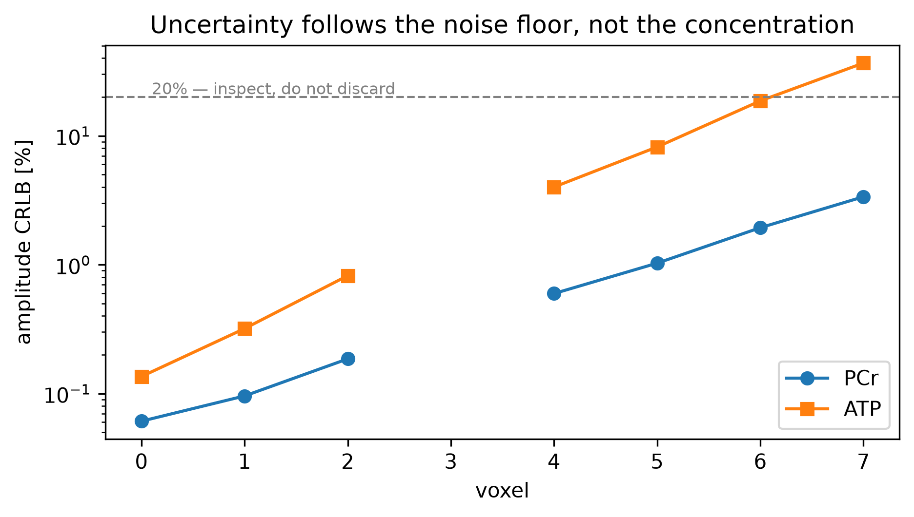
Did it follow the drift?¶
The second check is one the CRLB cannot give you: whether the fit found the peaks where they actually were. We know the answer, because we put the drift there.
fig, ax = plt.subplots(figsize=(7, 3.5))
ax.plot(ds["voxel"], b0_drift, "k--", lw=1, label="simulated B0 drift")
ds["chem_shift"].sel(metabolite="PCr").plot(ax=ax, marker="o", ls="none", label="fitted PCr")
(ds["chem_shift"].sel(metabolite="ATP") + 7.5).plot(
    ax=ax, marker="s", ls="none", label="fitted ATP (+7.5 ppm)"
)
ax.set_ylabel("shift from nominal [ppm]")
ax.set_title("Both peaks were tracked across the drift")
ax.legend()
plt.show()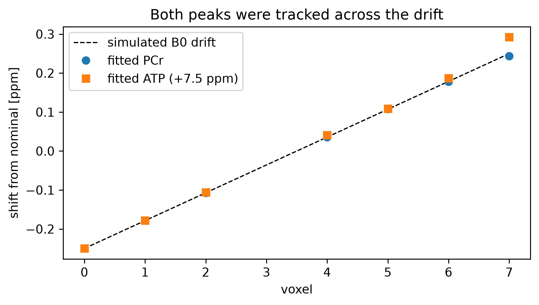
Each peak was found within a hundredth of a ppm of where it was put — including in the noisiest voxels, where the amplitude has already become uncertain. Position is a much better-conditioned quantity than area, which is worth remembering when a fit “looks bad”.
Look at the spectrum¶
The last check is the one no summary statistic replaces. data, fit and residuals come back in
the same domain you passed in, so plotting them is the same code for the best and worst voxel:
fig, axes = plt.subplots(1, 2, figsize=(11, 4), sharex=True)

for ax, v in zip(axes, [0, 7]):
    voxel = ds.isel(voxel=v)
    offset = -0.25 * float(np.abs(voxel["data"].xmr.to_spectrum().real).max())
    for var, color, label in (
        ("data", "black", "data"),
        ("fit", "tab:red", "fit"),
    ):
        voxel[var].xmr.to_spectrum().xmr.to_ppm().real.plot(
            ax=ax, color=color, alpha=0.5 if var == "data" else 1.0, label=label
        )
    (voxel["residuals"].xmr.to_spectrum().xmr.to_ppm().real + offset).plot(
        ax=ax, color="tab:green", lw=0.8, label="residual (offset)"
    )
    crlb = float(voxel["crlb"].sel(metabolite="ATP", parameter="amplitude"))
    ax.set_title(f"voxel {v} — ATP CRLB {crlb:.1f}%")
    ax.set_xlim(4, -12)
    ax.set_ylabel("intensity [a.u.]")
    ax.legend(fontsize=8)

plt.tight_layout()
plt.show()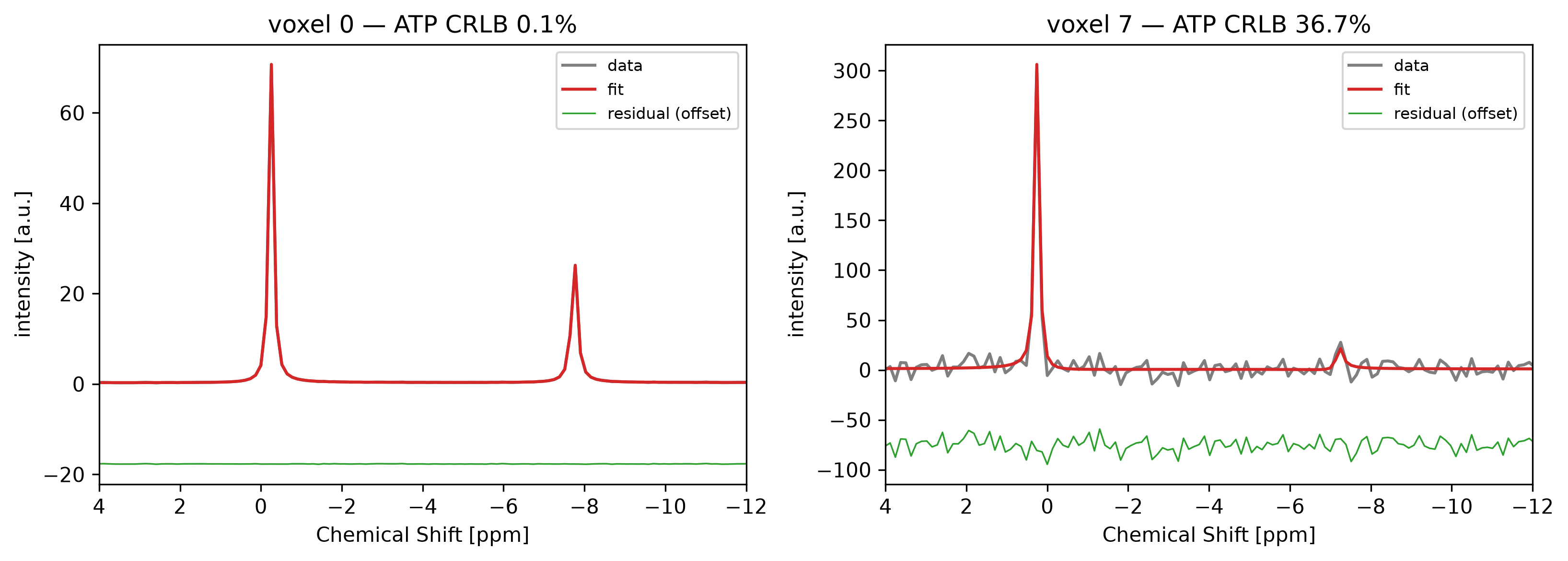
Both residuals are structureless — the model fits both voxels as well as the data allows. The difference between them is not fit quality, it is how much data there was. That distinction is exactly what a CRLB column tells you and a glance at a spectrum does not.
5. What holds when the data is real¶
The data above was synthetic, and synthetic data is forgiving in one specific way: it arrives at unit scale, in the domain the algorithm wants, with no missing voxels. Three guarantees cover what happens when it does not.
A non-answer is NaN, never 0 — shown in §3, with fit_status recording
which kind of absence it was.
Safe at any signal scale. A Bruker FID peaks around 1e7, and pyAMARES derives its optimizer
tolerance from signal magnitude — at that scale the tolerance balloons and the solver stops before
it has moved, handing back your prior guess dressed as a result. fit_amares normalizes the array,
fits where the tolerance behaves, and rescales:
scanner_scale = (grid.isel(voxel=0) * 1e7).assign_attrs(grid.attrs)
ds_scaled = scanner_scale.xmr.fit_amares(pk)

print("unit scale :", ds["amplitude"].isel(voxel=0).values.round(4))
print("x 1e7      :", ds_scaled["amplitude"].values)
print("ratio      :", (ds_scaled["amplitude"] / ds["amplitude"].isel(voxel=0)).values)
unit scale : [10.0044 5.0007]
x 1e7 : [1.00044046e+08 5.00065711e+07]
ratio : [ 9999999.96602904 10000000.03301361]
Either domain in, the same domain out. AMARES fits the FID, but you rarely hold one — you hold
a phased spectrum in ppm. Hand that over and fit_amares round-trips it for you, returning
data, fit and residuals in the representation you passed:
as_ppm = grid.isel(voxel=0).xmr.to_spectrum().xmr.to_ppm()
ds_ppm = as_ppm.xmr.fit_amares(pk)

print("fitted from a FID     :", ds["amplitude"].isel(voxel=0).values.round(4))
print("fitted from a spectrum:", ds_ppm["amplitude"].values.round(4))
print("signals came back on  :", ds_ppm["fit"].dims)
fitted from a FID : [10.0044 5.0007]
fitted from a spectrum: [10.0044 5.0007]
signals came back on : ('chemical_shift',)
- Xu, J., Vaeggemose, M., Schulte, R. F., Yang, B., Lee, C.-Y., Laustsen, C., & Magnotta, V. A. (2024). PyAMARES, an Open-Source Python Library for Fitting Magnetic Resonance Spectroscopy Data. Diagnostics, 14(23), 2668. 10.3390/diagnostics14232668
- Kreis, R. (2015). The trouble with quality filtering based on relative <scp>C</scp>ramér<scp>R</scp>ao lower bounds. Magnetic Resonance in Medicine, 75(1), 15–18. 10.1002/mrm.25568
- Wilson, M., Andronesi, O., Barker, P. B., Bartha, R., Bizzi, A., Bolan, P. J., Brindle, K. M., Choi, I., Cudalbu, C., Dydak, U., Emir, U. E., Gonzalez, R. G., Gruber, S., Gruetter, R., Gupta, R. K., Heerschap, A., Henning, A., Hetherington, H. P., Huppi, P. S., … Howe, F. A. (2019). Methodological consensus on clinical proton MRS of the brain: Review and recommendations. Magnetic Resonance in Medicine, 82(2), 527–550. 10.1002/mrm.27742