Apodization (windowing) lets you trade off between SNR and spectral resolution when processing FID signals. Choosing the right line broadening (LB) or Gaussian broadening (GB) parameters typically requires visual trial and error.
The xmris apodization widget lets you adjust these parameters with sliders and immediately see the effect on both the time and frequency domains.
For background on the underlying filter functions and their mathematical definitions, see the Apodization processing guide.
import matplotlib.pyplot as plt
import xarray as xr

import xmris
from xmris import simulate_fid
1. Generate Synthetic Data
We create a noisy FID with two closely spaced peaks to demonstrate resolution enhancement.
Source
da_fid = simulate_fid(
    amplitudes=[10.0, 8.0],
    frequencies=[150.0, 165.0],
    dampings=[15.0, 15.0],
    reference_frequency=298.0,
    carrier_ppm=4.7,
    spectral_width=2000.0,
    n_points=2048,
    target_snr=15.0,
)
2. Launch the Widget
Pass a 1D time-domain DataArray to the apodize method. The widget computes the Fourier transform in the browser and renders the FID (top) and spectrum (bottom) side by side.
da_fid.xmr.widget.apodize(
    unit="hz",
    lb_range=(0, 20.0),
    gb_range=(0, 30.0),
)Widget Controls
| Control | Description |
|---|---|
| Method | Switch between Exponential (SNR enhancement) and Lorentz-Gauss (resolution enhancement). See the Apodization guide for details on each filter. |
| Display Mode | Show the Real, Imaginary, or Magnitude spectrum. |
| Show Original | Overlay the un-apodized data as a gray trace for comparison. |
| LB / GB Sliders | Adjust apodization parameters. The orange dashed line on the FID canvas shows the weighting envelope being applied. |
3. Extract and Apply Parameters
Once you are satisfied with the result, click Close. The widget displays a copyable Python snippet so your parameters are recorded in your notebook.
Paste the generated code into the next cell:
# Pasted directly from the widget completion screen
da_apodized = da_fid.xmr.apodize_lg(lb=5.20, gb=6.00)

fig, ax = plt.subplots(figsize=(8, 3))
da_fid.xmr.to_spectrum().real.plot(ax=ax, color="gray", label="Original")
da_apodized.xmr.to_spectrum().real.plot(ax=ax, color="tab:blue", label="Apodized")
ax.set_title("Spectrum Processed via Widget Parameters")
ax.set_xlim(100, 220)
ax.legend()
plt.show()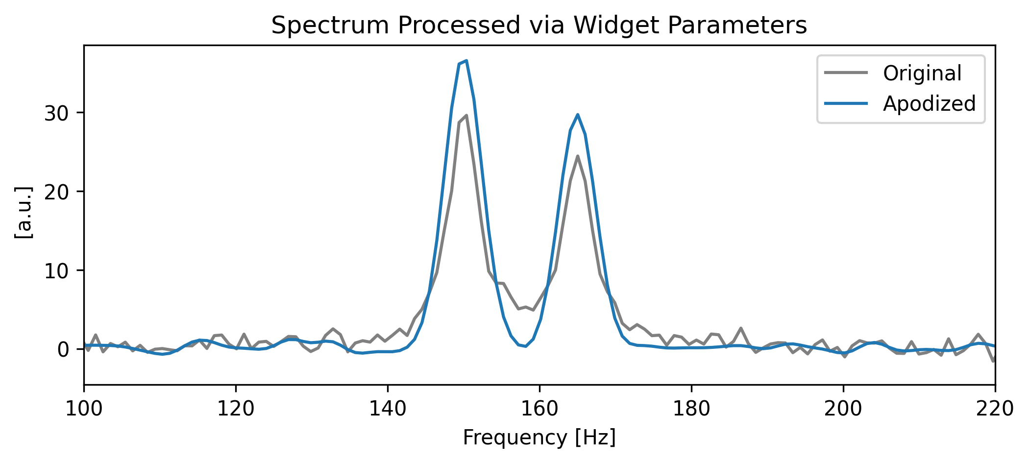
How the widget works internally
Unlike phase correction, which rotates complex numbers already in the frequency domain, apodization is applied in the time domain but must be evaluated in the frequency domain. Every slider adjustment requires the widget to:
Recalculate the weighting envelope.
Multiply it against the FID.
Perform a full FFT and fftshift.
Re-render both canvases.
To keep this responsive without a live Jupyter kernel, the widget includes a dependency-free, pure-JavaScript implementation of the Cooley-Tukey Radix-2 FFT algorithm that runs the entire DSP pipeline in the browser.
Automatic zero-filling. The Radix-2 algorithm requires input lengths that are powers of two. If your FID has a different length (e.g., 1000 points), the Python backend automatically zero-fills to the next power of two (e.g., 1024). This is mathematically equivalent to interpolation in the frequency domain and does not introduce artifacts.