Waterfall Plots

Waterfall plots (also known as ridge or joy plots) are essential in Magnetic Resonance Spectroscopy (MRS) for visualizing kinetic, dynamic, or relaxation series. By vertically stacking and horizontally offsetting 1D spectra, they allow the human eye to easily track peak growth, decay, and frequency shifts over an independent variable like time .

In xmris, this visualization is built entirely around our WaterfallConfig object, giving you publication-ready results without cluttering your function calls.

1. Data Requirements¶

Before plotting, your xarray.DataArray must meet the following criteria:

• Dimensionality: Must be at least 2D.

• X-Axis (Horizontal): The accessor will automatically search for dimensions named chemical_shift or frequency. If your spectral axis has a different name, you must specify it explicitly via the x_dim argument.

• Stack Axis (Vertical): The accessor will automatically stack along the remaining dimension. If multiple dimensions remain, it looks for averages or repetitions, or you can specify it explicitly via the stack_dim argument.

2. Generating Synthetic Data¶

We will generate a realistic kinetic time-course of a hyperpolarized 13C experiment where Pyruvate decays and Lactate grows over 60 seconds.

import numpy as np
import xarray as xr
import matplotlib.pyplot as plt

from xmris.fitting.simulation import simulate_fid
from xmris.visualization import WaterfallConfig

# Define our time series
time_points = np.linspace(0, 60, 25)
fids = []

# Simulate the kinetic evolution
for t in time_points:
    pyr_amp = 1000.0 * np.exp(-t / 20.0)
    lac_amp = 400.0 * (1.0 - np.exp(-t / 20.0))

    fid = simulate_fid(
        amplitudes=[lac_amp, pyr_amp],
        chemical_shifts=[183.3, 171.0],
        reference_frequency=32.1,
        carrier_ppm=171.0,
        spectral_width=5000.0,
        n_points=1024,
        dampings=[10.0, 12.0],
        phases=[0.0, 0.0],
        lineshape_g=[0.0, 0.0],
        target_snr=25.0
    )
    fids.append(fid)

# Combine into a 2D array by stacking along a new 'kinetic_time' dimension
da_kinetic_fid = xr.concat(fids, dim="kinetic_time").assign_coords(kinetic_time=time_points)
da_kinetic_fid.coords["kinetic_time"].attrs["units"] = "s"

# Convert to frequency-domain spectrum (ppm) and extract the real part
da_kinetic = da_kinetic_fid.xmr.to_spectrum().xmr.to_ppm().real

3. Basic Usage¶

Because we utilize an intelligent xarray accessor, the simplest plotting call requires zero arguments. The accessor dynamically reads the dataset’s units and dimensions to build the axes automatically.

# We slice the region of interest, and the accessor handles the rest
ax = da_kinetic.sel(chemical_shift=slice(160, 190)).xmr.plot.waterfall()
plt.show()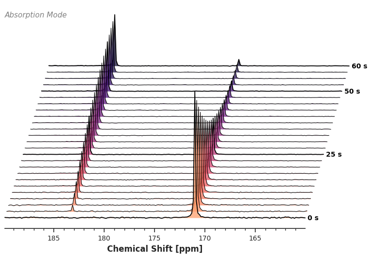

4. Advanced Configuration¶

To customize the plot, do not pass endless keyword arguments. Instead, instantiate a WaterfallConfig. Outputting this object in a notebook renders a table of all available styling options.

CFG = WaterfallConfig()
CFG

You can update these parameters using standard attribute assignment. Let’s create a dynamic, pseudo-3D angled sheer with heavy overlap.

CFG.stack_scale = 10.0
CFG.stack_offset = 0.5
CFG.stack_skew = -20.0
CFG.cmap = "viridis"
CFG.annotation = None
CFG.xlabel = r"$^{13}\mathrm{C}$ Chemical Shift"

# Pass the config to the accessor
ax = da_kinetic.sel(chemical_shift=slice(160, 190)).xmr.plot.waterfall(config=CFG)
plt.show()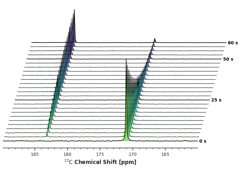

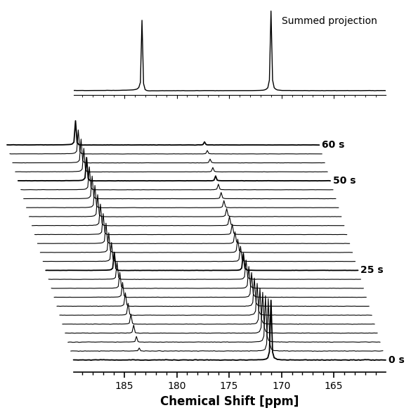
5. Subplot Integration (Wireframe Mode)¶

Professional library functions should never hijack your global plotting environment. Because plot.waterfall() returns a standard matplotlib.Axes object and accepts an ax keyword argument, you can easily embed these visualizations into multi-panel figures.

Here, we also demonstrate the Wireframe Mode by setting cmap=None, which disables the filled polygons for a clean, minimalist look.

from matplotlib.offsetbox import AnchoredText

# Configure a wireframe plot
CFG_WIRE = WaterfallConfig(
    cmap=None,  # Disables fill_between
    annotation=None,
    stack_scale=10.0,
    stack_offset=1.5,
    stack_skew=10.0
)

# Create a custom multi-panel figure
fig, (ax_top, ax_bottom) = plt.subplots(
    nrows=2,
    figsize=(6, 6),
    gridspec_kw={"height_ratios": [1, 3]},
    sharex=True,
)

# 1. Plot a standard 1D summed spectrum on the top panel
da_kinetic.sel(chemical_shift=slice(160, 190)).sum(dim="kinetic_time").plot.line(ax=ax_top, color="black", linewidth=1)

text_box = AnchoredText("Summed projection", loc="upper right", frameon=False, prop=dict(fontsize=10))
ax_top.add_artist(text_box)
ax_top.invert_xaxis()
ax_top.set_xlabel("")
ax_top.set_ylabel("")
ax_top.set_yticks([])
for spine in ["left", "right", "top"]:
    ax_top.spines[spine].set_visible(False)

# 2. Inject the waterfall plot into the bottom panel
_ = da_kinetic.sel(chemical_shift=slice(160, 190)).xmr.plot.waterfall(ax=ax_bottom, config=CFG_WIRE)

plt.tight_layout()
plt.show()

# STRICT TESTS FOR CI
assert isinstance(ax_bottom, plt.Axes), "plot.waterfall must return a matplotlib Axes object."

# Ensure the wireframe mode worked (no collections, but lines exist)
assert len(ax_bottom.collections) == 0, "Colormap was None, but filled areas were generated."
assert len(ax_bottom.lines) > 0, "No outline lines were plotted in wireframe mode."

x_label = ax.get_xlabel()
assert "13" in x_label and "C" in x_label, "Chemical shift LaTeX formatting failed on the colored plot."

# Verify xarray lineage is preserved
assert "kinetic_time" in da_kinetic.dims, "Time dimension was lost during processing."
assert "chemical_shift" in da_kinetic.dims, "Chemical shift dimension was lost."