Carpet Plots

As a quantitative alternative to the 2D waterfall plot (see 2. Waterfall Plots), carpet plots provide a top-down, 2D image representation of stacked spectra . They are 2D rasterized visualizations of 1D time-series data, effectively “rolling out” the time-domain flat on the floor. This approach eliminates visual occlusion, allowing for direct observation of signal intensities and frequency shifts across the stacking dimension (e.g., time or repetitions).

In xmris, this visualization is built around the CarpetConfig object, which includes specialized logic for truncating colormaps so your data never gets lost in absolute white or absolute black on printed paper.

1. Data Requirements¶

Before plotting, your xarray.DataArray must meet the following criteria:

Dimensionality: Must be at least 2D.
X-Axis (Horizontal): The accessor automatically searches for chemical_shift or frequency.
Y-Axis (Vertical): The accessor automatically assigns the remaining dimension to the y-axis (e.g., kinetic_time or averages).

2. Generating Synthetic Data¶

To ensure a 1:1 comparison with the waterfall plot, we will generate the exact same synthetic kinetic time-course. We simulate a hyperpolarized 13C experiment where Pyruvate decays and Lactate grows over 60 seconds.

We will use the xmris.fitting.simulation module:

import numpy as np
import xarray as xr
import matplotlib.pyplot as plt

from xmris.fitting.simulation import simulate_fid
from xmris.visualization import CarpetConfig, WaterfallConfig

# Define our time series
time_points = np.linspace(0, 60, 25)
fids = []

# Simulate the kinetic evolution
for t in time_points:
    pyr_amp = 1000.0 * np.exp(-t / 20.0)
    lac_amp = 400.0 * (1.0 - np.exp(-t / 20.0))

    fid = simulate_fid(
        amplitudes=[lac_amp, pyr_amp],
        chemical_shifts=[183.3, 171.0],
        reference_frequency=32.1,
        carrier_ppm=171.0,
        spectral_width=5000.0,
        n_points=1024,
        dampings=[10.0, 12.0],
        phases=[0.0, 0.0],
        lineshape_g=[0.0, 0.0],
        target_snr=25.0
    )
    fids.append(fid)

# Combine into a 2D array by stacking along a new 'kinetic_time' dimension
da_kinetic_fid = xr.concat(fids, dim="kinetic_time").assign_coords(kinetic_time=time_points)
da_kinetic_fid.coords["kinetic_time"].attrs["units"] = "s"

# Convert to frequency-domain spectrum (ppm) and extract the real part
da_kinetic = da_kinetic_fid.xmr.to_spectrum().xmr.to_ppm().real

3. Basic Usage¶

Because plot.carpet() shares the same intelligent dimension parser as plot.waterfall(), you can call it without any dimension arguments.

# We slice the region of interest, and the accessor handles the rest
ax = da_kinetic.sel(chemical_shift=slice(160, 190)).xmr.plot.carpet()
plt.show()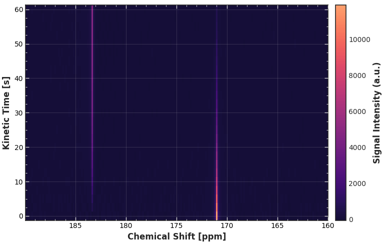

4. Advanced Configuration¶

Instantiating the CarpetConfig reveals specialized controls for the 2D grid. Notice how the default setting (grid_on=True) utilizes a subtle overlaid grid and inward-facing ticks to make reading exact coordinates effortless.

CFG_CARPET = CarpetConfig()
CFG_CARPET

We can customize the labels and adjust the colormap boundaries to make the contrast pop.

CFG_CARPET.xlabel = r"$^{13}\mathrm{C}$ Chemical Shift"
CFG_CARPET.cmap = "inferno"
CFG_CARPET.cmap_start = 0.05
CFG_CARPET.cmap_end = 0.95

# Plot using the accessor
ax = da_kinetic.sel(chemical_shift=slice(160, 190)).xmr.plot.carpet(config=CFG_CARPET)
plt.show()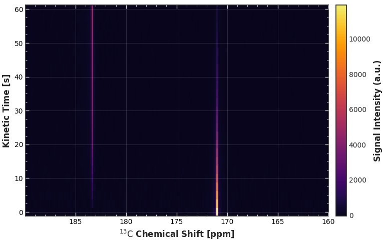

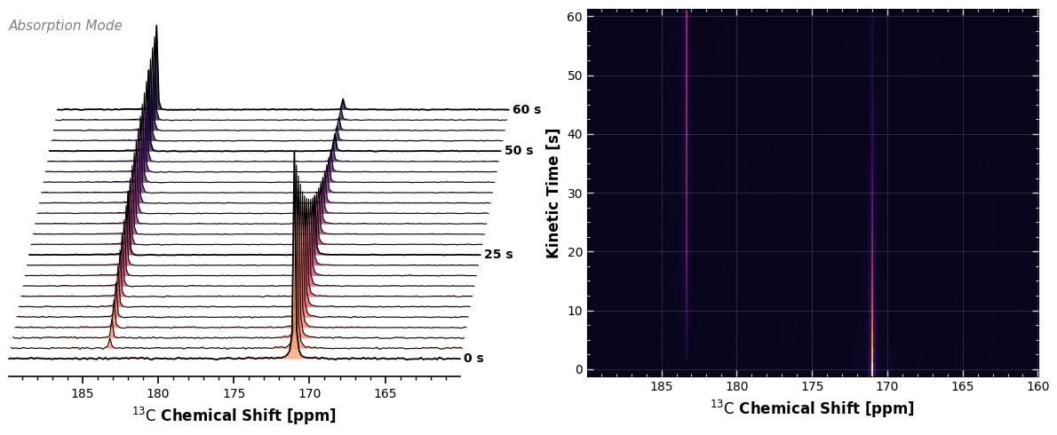
5. Subplot Integration¶

Because our plotting functions return standard matplotlib.Axes objects, we can easily build a comprehensive, multi-panel figure combining the qualitative intuition of the Waterfall Plot with the quantitative rigor of the Carpet Plot.

# Setup the Waterfall configuration
CFG_WATERFALL = WaterfallConfig(
    xlabel=r"$^{13}\mathrm{C}$ Chemical Shift", 
    annotation="Absorption Mode",
    stack_skew=-15.0
)

# Turn off the colorbar on the carpet to save horizontal space
CFG_CARPET.cbar_on = False  

# Create a 1x2 grid
fig, (ax_left, ax_right) = plt.subplots(
    nrows=1, ncols=2, figsize=(12, 5), gridspec_kw={"width_ratios": [1, 1]}
)

# Render Waterfall on the left, Carpet on the right
da_kinetic.sel(chemical_shift=slice(160, 190)).xmr.plot.waterfall(ax=ax_left, config=CFG_WATERFALL)
da_kinetic.sel(chemical_shift=slice(160, 190)).xmr.plot.carpet(ax=ax_right, config=CFG_CARPET)

plt.tight_layout()
plt.show()

# STRICT TESTS FOR CI
assert isinstance(ax_right, plt.Axes), "plot.carpet must return a matplotlib Axes object."
assert len(ax_right.collections) > 0, "No pcolormesh was generated by the carpet."

x_label = ax_right.get_xlabel()
assert "13" in x_label and "C" in x_label, "Chemical shift LaTeX formatting failed on the carpet plot."

# Verify xarray lineage is preserved
assert "kinetic_time" in da_kinetic.dims, "Time dimension was lost during processing."
assert "chemical_shift" in da_kinetic.dims, "Chemical shift dimension was lost."