Asymmetric Least Squares (AsLS) Baseline Correction

Magnetic Resonance Spectroscopy (MRS) signals often ride on top of a broad, rolling baseline. This distortion is typically caused by macromolecules with extremely short $T_2$ relaxation times (creating very broad frequency-domain peaks), acoustic ringing, or incomplete water suppression.

To accurately quantify the sharp, narrow metabolite peaks, this baseline must be mathematically isolated and removed.

The Mathematics of AsLS¶

In xmris, we use the Asymmetric Least Squares (AsLS) algorithm introduced by Eilers & Boelens (2005). Unlike simple polynomial fitting, AsLS does not require the user to manually define “signal-free” noise regions. Instead, it balances two competing goals: minimizing the distance between the experimental data and the baseline, and maximizing the smoothness of the baseline itself.

It minimizes the following penalized least-squares objective function:

S = \sum_i w_i (y_i - z_i)^2 + \lambda \sum_i (\Delta^2 z_i)^2

(1)

Where:

$y$ is the experimental spectrum.
$z$ is the fitted baseline curve.
$\lambda$ (Lambda) is the smoothness penalty. A higher $\lambda$ yields a stiffer, flatter baseline.
$w$ is the asymmetric weighting factor.

The asymmetry is governed by a parameter $p$ (typically between 0.001 and 0.05). The algorithm iteratively updates the weights: if a data point is above the baseline (a peak), it is given a tiny weight ( $p$ ). If it is below the baseline, it is given a large weight ( $1-p$ ). This forces the curve to aggressively hug the bottom of the signal, naturally slipping under the narrow absorption peaks.

1. Generating Synthetic Data¶

Let’s simulate a complex FID with two sharp metabolite peaks and one massive, heavily damped macromolecular peak acting as our rolling baseline.

import numpy as np
import matplotlib.pyplot as plt
import xarray as xr
import xmris

# Import xmris core vocabularies and our simulation tool
from xmris.core.config import DIMS, COORDS, ATTRS
from xmris import simulate_fid

# Simulated spectrometer parameters
SW = 2000.0  # Hz
N = 1024
REF_FREQ = 123.2  # 3T Phosphorus (MHz)

# 1. Sharp metabolites (low damping)
fid_metabs = simulate_fid(
    amplitudes=[10.0, 5.0],
    chemical_shifts=[5.0, -2.5],
    dampings=[30.0, 40.0], # Narrow, long-lived signals
    reference_frequency=REF_FREQ,
    spectral_width=SW,
    n_points=N
)

# 2. Realistic rolling baseline
# A superposition of ultra-short T2 components spanning the spectrum
fid_macro = simulate_fid(
    amplitudes=[35.0, 45.0, 30.0],
    chemical_shifts=[3.0, 0.5, -1.5],
    dampings=[1200.0, 1800.0, 1500.0], # Extreme dampings smear these into a wave
    reference_frequency=REF_FREQ,
    spectral_width=SW,
    n_points=N,
    target_snr=40 # Realistic noise
)

# Combine for final simulated signal
fid_total = fid_metabs + fid_macro

# Preserve lineage from the simulation
fid_total.attrs = fid_metabs.attrs.copy()

2. Applying AsLS via the xmris Accessor¶

Because xmris baseline correction strictly operates on frequency-domain absorption peaks, we must first Fourier transform the signal using the to_spectrum() accessor method. Once in the frequency domain, we can seamlessly chain our baseline correction.

# 1. Transform FID to a centered Frequency-Domain spectrum
spectrum = fid_total.xmr.to_spectrum()

# 2. Apply xmris AsLS Baseline Correction via the fluent API
# Note: This automatically isolates the real part and safely preserves attributes!
corrected_spectrum = spectrum.xmr.baseline_als(
    lam=1e5,
    p=0.01
)

Visualizing the Results¶

Let’s look at the original real spectrum, the isolated baseline, and the final corrected spectrum.

fig, ax = plt.subplots(figsize=(10, 5))

# Calculate the baseline (xarray handles the math and metadata continuity)
estimated_baseline = spectrum.real - corrected_spectrum

# Use xarray's native plotting! It automatically reads coordinates and metadata.
spectrum.real.plot(ax=ax, label="Original Real Spectrum", color="#cfd8dc")
estimated_baseline.plot(ax=ax, label="Estimated AsLS Baseline", color="#ef5350", linestyle="--")
corrected_spectrum.plot(ax=ax, label="Corrected Spectrum", color="#1976d2", linewidth=1.5)

# Standard NMR convention (reverse axis)
ax.set_xlim(1000, -1000)

# Clean up the visual presentation
ax.set_title("AsLS Baseline Correction")
ax.legend()
ax.grid(alpha=0.3)
plt.show()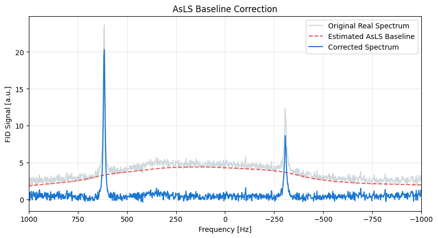

# --- HIDDEN CI TESTS ---

# 1. Purity Check: Original array is unmodified
assert np.iscomplexobj(spectrum), "Original spectrum was improperly mutated to real."

# 2. Type Check: Corrected array is strictly real
assert not np.iscomplexobj(corrected_spectrum), "Corrected spectrum contains imaginary data!"

# 3. Lineage Check: Old attributes survived, new attributes appended via accessor
assert ATTRS.reference_frequency in corrected_spectrum.attrs
assert corrected_spectrum.attrs[ATTRS.baseline_method] == "als"
assert corrected_spectrum.attrs[ATTRS.baseline_lam] == 1e5
assert corrected_spectrum.attrs[ATTRS.baseline_p] == 0.01

# 4. Math Check: Test a "metabolite-free" region (e.g., 1.0 ppm)
# 1.0 ppm * 123.2 MHz = 123.2 Hz. This region should be pure baseline.
freqs = spectrum.coords[DIMS.frequency].values
center_idx = int(np.argmin(np.abs(freqs - 123.2)))

orig_val = float(spectrum.real.values[center_idx])
corr_val = float(corrected_spectrum.values[center_idx])

# Check 1: Ensure the simulated rolling baseline actually has power here
assert orig_val > 0.5, f"Original data missing baseline signal. Value: {orig_val}"

# Check 2: Scale-invariant suppression. Since this region is pure baseline,
# AsLS should have flattened it out, reducing the signal by at least 80%.
assert np.abs(corr_val) < (0.2 * np.abs(orig_val)), (
    f"Baseline not sufficiently removed! Original: {orig_val:.2f}, "
    f"Corrected: {corr_val:.2f}"
)

References¶

Eilers, P. H., & Boelens, H. F. (2005). Baseline correction with asymmetric least squares smoothing (Report No. 1; Vol. 1, p. 5). Leiden University Medical Centre.