Goal: Visually verify the strict 1D-to-ND Bruker memory reshaping, physical coordinate calculation, and the newly refactored xmris processing pipeline. We will explicitly use xarray’s native plotting to ensure units and axis names are automatically and correctly resolved.
from pathlib import Path
import xarray as xr

from xmris.vendor.bruker import reshape_bruker_raw, build_fid
from xmris.core.config import DIMS, COORDS

# Configuration
xr.set_options(display_expand_data=False)
<xarray.core.options.set_options at 0x7f53a37ef290>1. Data Loading and Reshaping
Raw Bruker data is read as a continuous 1D array. To make it useful, we must reshape it into an N-dimensional C-contiguous array based on the acquisition parameters, and then wrap it in an xarray.DataArray with the correct physical coordinates.
DATA_DIR = Path("../../../tests/data/")
FILE_PATH = Path(DATA_DIR / "nspect_slab_1H" / "rawdatajob0.nc")

# Load the raw 1D complex data
raw_1d_data = xr.load_dataarray(FILE_PATH).xmr.to_complex()

# Reshape into C-contiguous N-dimensional numpy array
reshaped_nd, valid_dims = reshape_bruker_raw(raw_1d_data.values, raw_1d_data.attrs)

# Construct the FID DataArray
fid_xr = build_fid(reshaped_nd, valid_dims, raw_1d_data.attrs)

print(f"Constructed FID Shape: {fid_xr.shape}")
print(f"Assigned Attributes: {list(fid_xr.attrs.keys())}")
Reshaped Bruker data to dims: [ time | averages ]
Constructed FID Shape: (2048, 5)
Assigned Attributes: ['reference_frequency', 'carrier_ppm', 'bruker_group_delay', 'units']
2. Inspecting the Time Domain (FID)
To simplify our visual inspection, we will select the first repetition, channel, or average if the data is multi-dimensional. We then plot the Free Induction Decay (FID) to verify signal decay shape, complex quadrature, and the absence of truncation artifacts.
# Select a 1D slice for basic visual inspection if multi-dimensional
if fid_xr.ndim > 1:
    fid_inspect = fid_xr.isel({d: 0 for d in fid_xr.dims if d != DIMS.time})
else:
    fid_inspect = fid_xr

fig, ax = plt.subplots(figsize=(10, 4))

# Use xarray's native plotting to verify automatic labels
fid_inspect.real.plot(ax=ax, label="Real", alpha=0.8)
fid_inspect.imag.plot(ax=ax, label="Imaginary", alpha=0.8)

ax.set_title("Time Domain: Raw FID")
ax.legend()
ax.grid(True, alpha=0.3)

plt.show()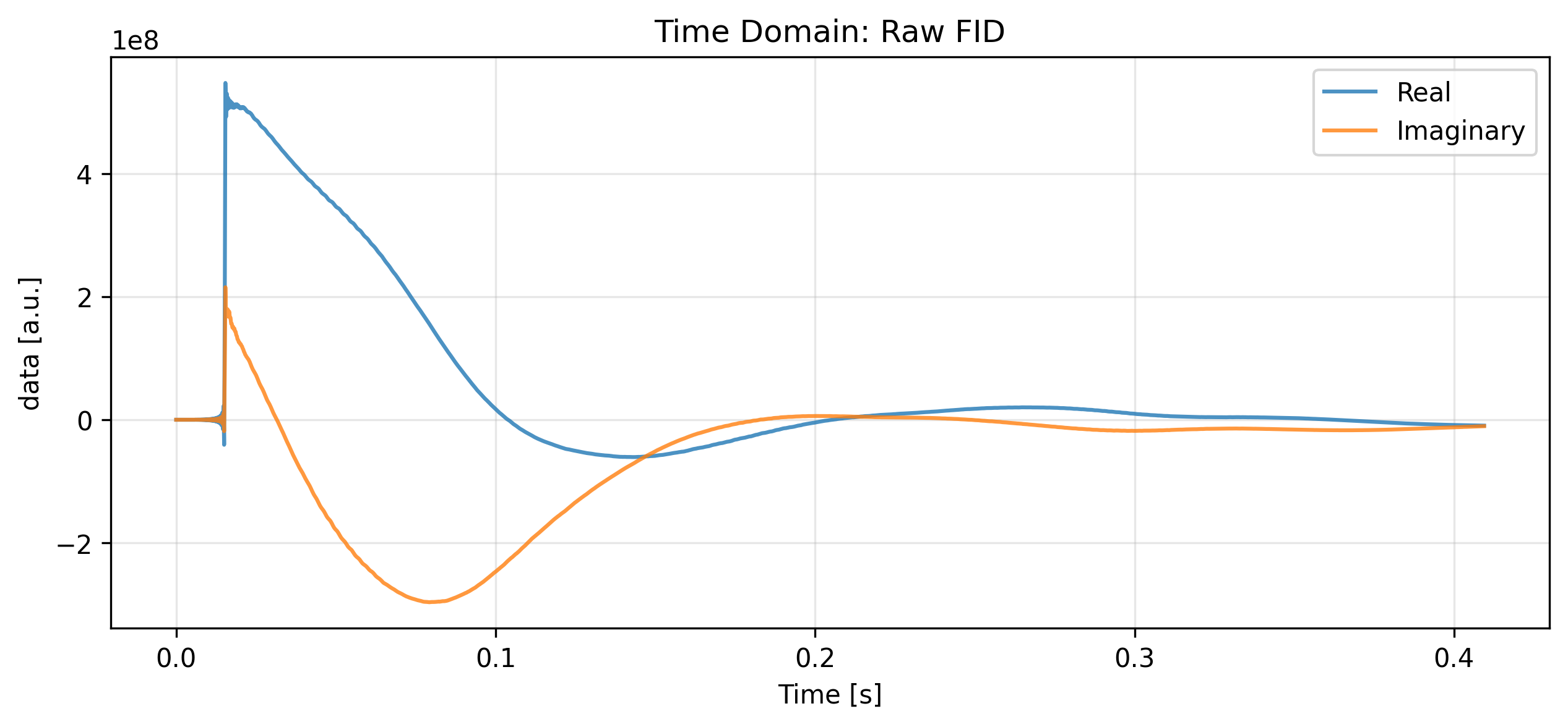
Removing the Digital Filter
Bruker spectrometers utilize digital filters that introduce a group delay at the beginning of the FID. We use the remove_digital_filter accessor to correct this, relying on the groupDelay attribute from the metadata.
# Remove group delay
fid_corrected = fid_inspect.xmr.remove_digital_filter(
    group_delay=raw_1d_data.attrs["groupDelay"],
    keep_length=False
)

fig, ax = plt.subplots(figsize=(10, 4))

fid_corrected.real.plot(ax=ax, label="Real", alpha=0.8, marker='.')
fid_corrected.imag.plot(ax=ax, label="Imaginary", alpha=0.8, marker='.')

ax.set_title("Time Domain: Corrected FID (Group Delay Removed)")
ax.legend()
ax.grid(True, alpha=0.3)

plt.show()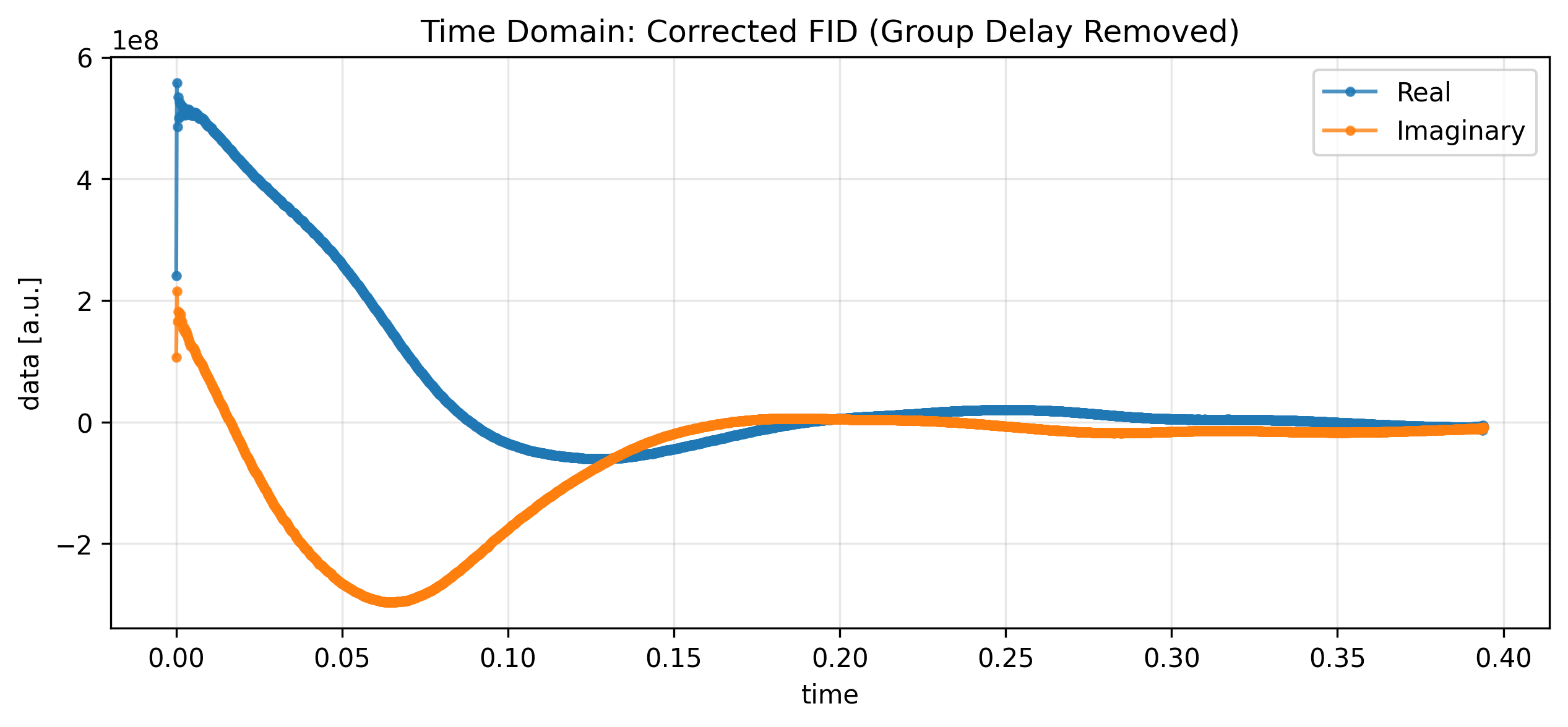
3. The xmris Spectral Pipeline
With the FID corrected, we can pass it through the xmris processing pipeline. Here, we apply an exponential apodization to smooth the signal, transform it to the frequency domain, and automatically correct the phase.
# Apply the strict xmris pipeline
spectrum = (
    fid_corrected
    # .xmr.apodize_exp(lb=2)
    .xmr.to_spectrum()
    .xmr.autophase()
)

spectrumVisualizing the Frequency Domain
We can visualize the resulting spectrum. Note how xarray automatically handles the coordinate labels. We invert the x-axis to adhere to standard NMR/MRI conventions.
fig, (ax1, ax2) = plt.subplots(2, 1, figsize=(10, 10))

# --- Subplot 1: Real Component ---
spectrum.real.plot(ax=ax1, color="red", marker='.')
ax1.set_title("Frequency Domain (Real)")
ax1.grid(True, alpha=0.3)
ax1.xaxis.set_inverted(True)

# --- Inlay Plot for Subplot 1 (Top Left) ---
# [x, y, width, height] in normalized axes coordinates (0 to 1)
axins = ax1.inset_axes([0.05, 0.55, 0.35, 0.35])
spectrum.real.plot(ax=axins, color="red", marker='.')

# Set limits for the zoom (x-axis inverted to match the main plot)
axins.set_xlim(100, -100)
axins.set_ylim(-1e8, 0.5e9) # Keeping a slight negative baseline so the peak doesn't float

# Clean up inset labels so it doesn't clutter the main plot
axins.set_title('')
axins.set_xlabel('')
axins.set_yticks([0, 0.5e9])
axins.set_ylabel('')
axins.grid(True, alpha=0.3)

# Draw connecting lines from the inset to the zoomed region
# ax1.indicate_inset_zoom(axins, edgecolor="black", alpha=0.5)

# --- Subplot 2: Imaginary Component ---
spectrum.imag.plot(ax=ax2, color="navy", marker='.')
ax2.set_title("Frequency Domain (Imaginary)")
ax2.grid(True, alpha=0.3)
ax2.xaxis.set_inverted(True)

plt.tight_layout()
plt.show()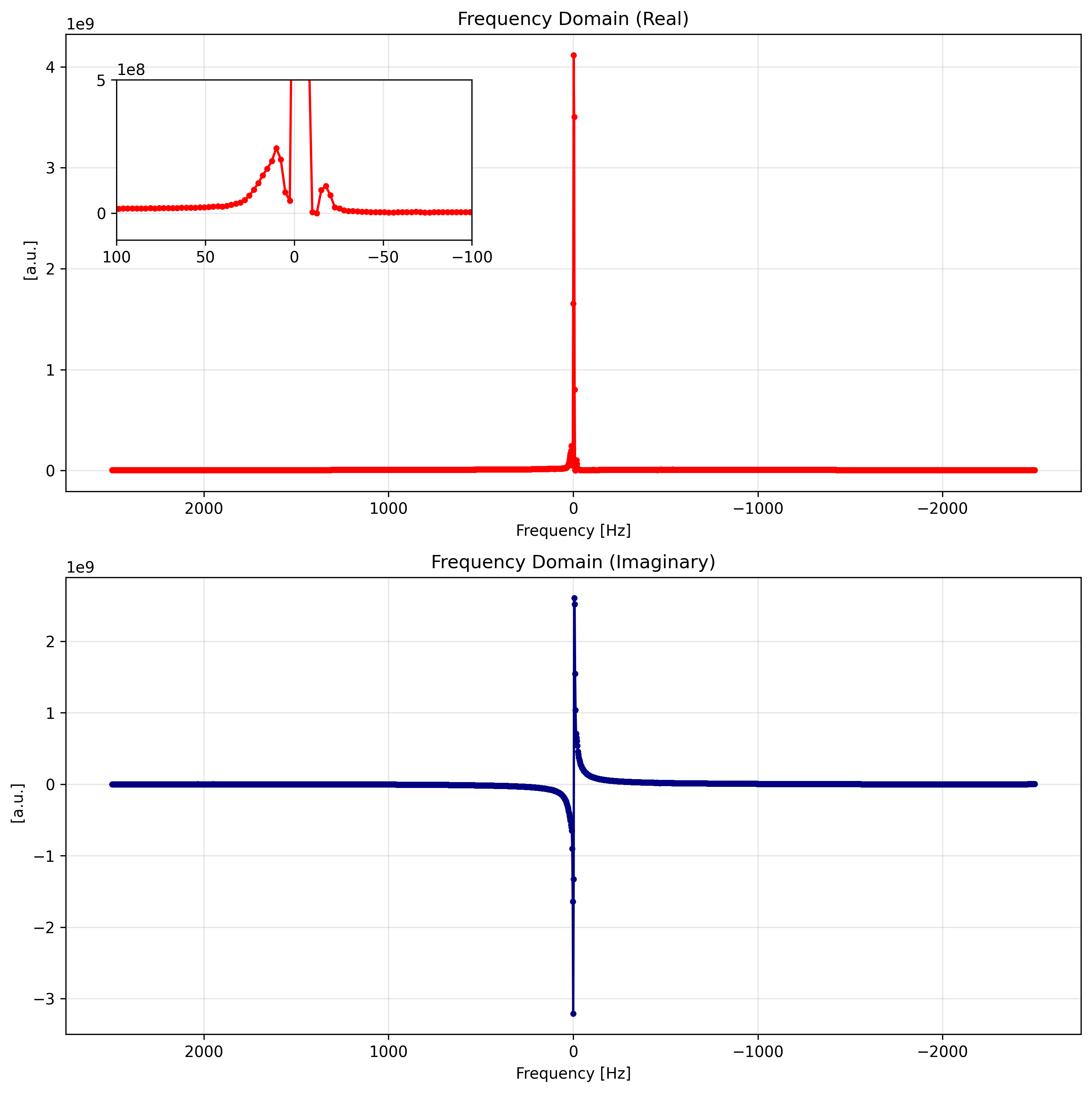
4. Chemical Shift Conversion
For chemical analysis, viewing the spectrum in parts per million (ppm) is more useful than raw Hertz. The .xmr.to_ppm() accessor handles this conversion automatically using the spectrometer frequency metadata.
# Convert frequency to chemical shift (ppm)
spectrum_ppm = spectrum.xmr.to_ppm()

fig, (ax1, ax2) = plt.subplots(2, 1, figsize=(10, 10))

# --- Subplot 1: Real Component ---
spectrum_ppm.real.plot(ax=ax1, color="red", marker='.')
ax1.set_title("Frequency Domain (Real)")
ax1.grid(True, alpha=0.3)
ax1.xaxis.set_inverted(True)

# --- Inlay Plot for Subplot 1 (Top Left) ---
# [x, y, width, height] in normalized axes coordinates (0 to 1)
axins = ax1.inset_axes([0.05, 0.55, 0.35, 0.35])
spectrum_ppm.real.plot(ax=axins, color="red", marker='.')

# Set limits for the zoom (x-axis inverted to match the main plot)
axins.set_xlim(5.7, 3.7)
axins.set_ylim(-1e8, 0.5e9) # Keeping a slight negative baseline so the peak doesn't float

# Clean up inset labels so it doesn't clutter the main plot
axins.set_title('')
axins.set_xlabel('')
axins.set_yticks([0, 0.5e9])
axins.set_ylabel('')
axins.grid(True, alpha=0.3)

# Draw connecting lines from the inset to the zoomed region
# ax1.indicate_inset_zoom(axins, edgecolor="black", alpha=0.5)

# --- Subplot 2: Imaginary Component ---
spectrum_ppm.imag.plot(ax=ax2, color="navy", marker='.')
ax2.set_title("Frequency Domain (Imaginary)")
ax2.grid(True, alpha=0.3)
ax2.xaxis.set_inverted(True)

plt.tight_layout()
plt.show()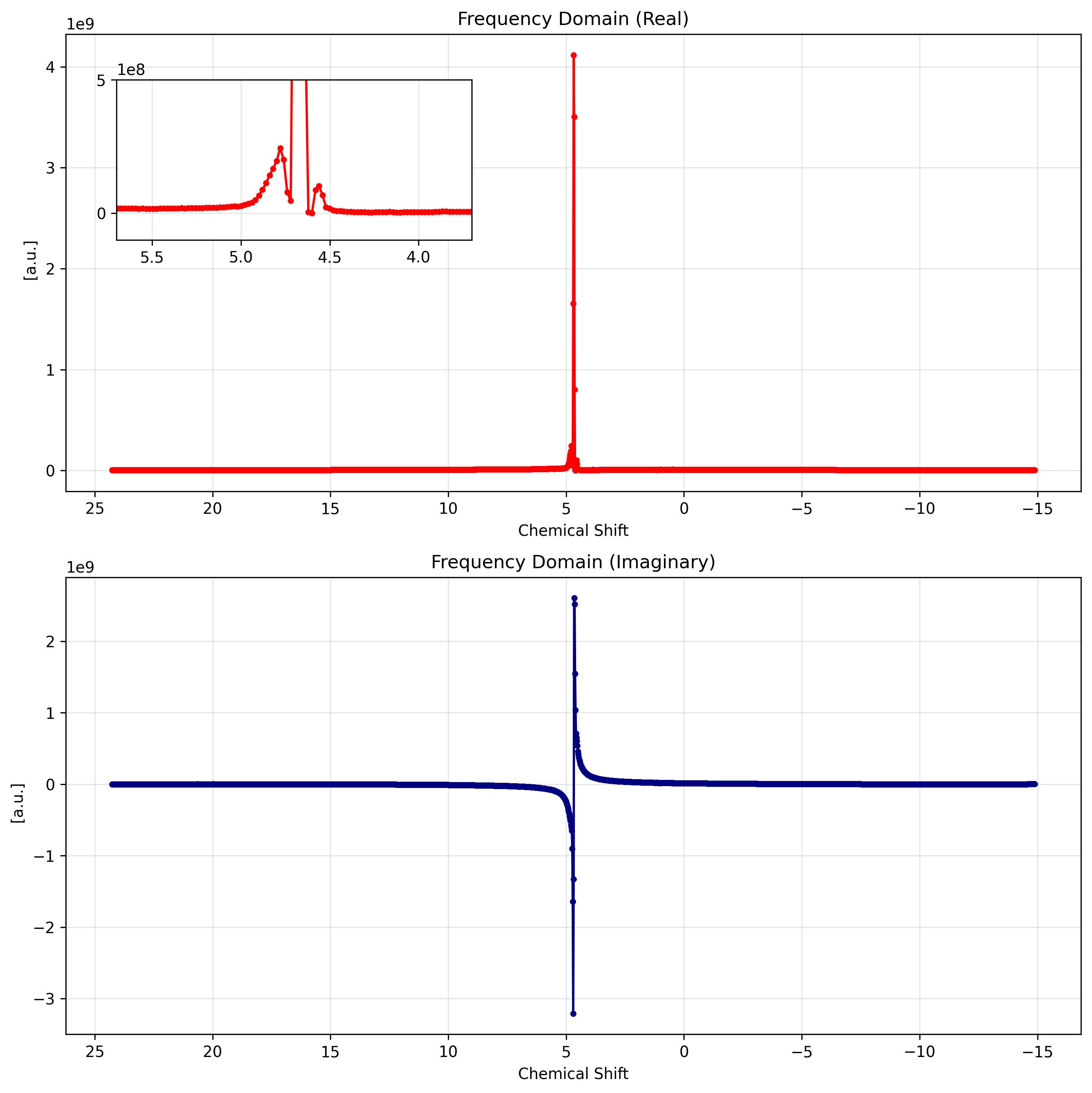
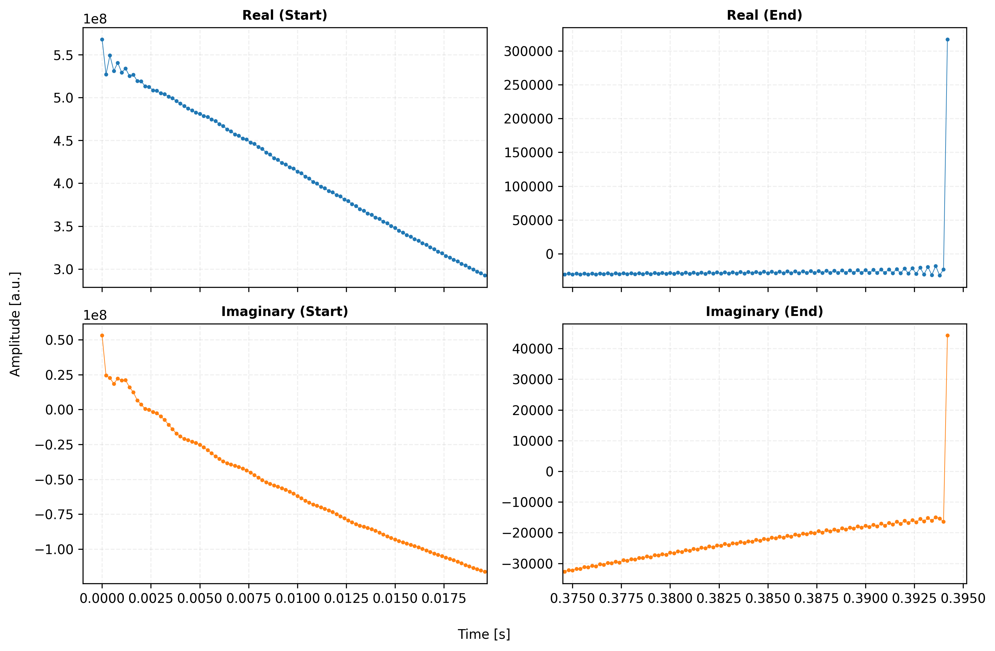
5. Reverse Transformation
The xmris accessors preserve metadata and coordinates perfectly, allowing seamless reverse transformations. We can convert our processed spectrum back into the time domain using .xmr.to_fid().
# Inverse Fourier Transform back to Time Domain
fid_final = spectrum.xmr.to_fid()

fig, ax = plt.subplots(figsize=(10, 4))

fid_final.real.plot(ax=ax, label="Real", alpha=0.8, marker='.')
fid_final.imag.plot(ax=ax, label="Imaginary", alpha=0.8, marker='.')

ax.set_title("Time Domain: Reconstructed FID")
ax.legend()
ax.grid(True, alpha=0.3)

plt.show()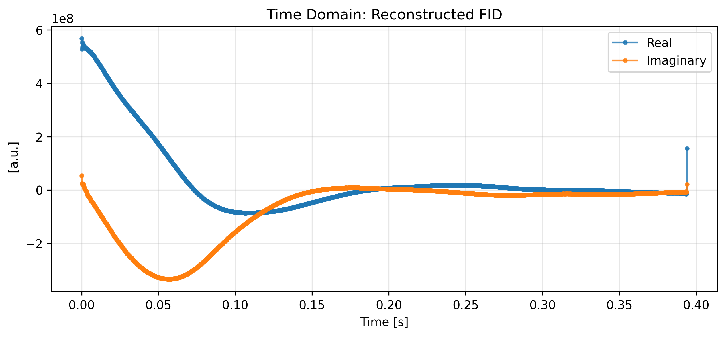
# --- Configuration: Easy Adjustments ---
view_cfg = {
    "zoom_percent": 0.05,    # Window size (5% of total FID)
    "padding_percent": 0.05  # 5% padding relative to the local data range
}

# 1. Transform back to Time Domain
fid_final = spectrum.xmr.to_fid()

# 2. Setup the 2x2 grid with shared axes for decluttering
# sharex='col' -> Top and Bottom share the same time window
# sharey='row' -> Left and Right share the same amplitude scale
fig, axes = plt.subplots(2, 2, figsize=(11, 7), sharex='col')
(ax_real_start, ax_real_end), (ax_imag_start, ax_imag_end) = axes

# --- Logic: Calculate Time Windows ---
t_coords = fid_final[fid_final.dims[0]]
t_min, t_max = float(t_coords.min()), float(t_coords.max())
t_total = t_max - t_min
window_len = t_total * view_cfg["zoom_percent"]

# Define the data slices for plotting
start_slice = fid_final.sel({fid_final.dims[0]: slice(t_min, t_min + window_len)})
end_slice = fid_final.sel({fid_final.dims[0]: slice(t_max - window_len, t_max)})

# --- Helper to calculate padded limits ---
def get_padded_limits(data, pad_frac):
    d_min, d_max = float(data.min()), float(data.max())
    d_range = d_max - d_min
    padding = (d_range * pad_frac) if d_range > 0 else 0.1
    return d_min - padding, d_max + padding

# --- Execute Plotting ---
# Row 1: Real
start_slice.real.plot(ax=ax_real_start, color="C0", marker='.', markersize=4, linewidth=0.5)
end_slice.real.plot(ax=ax_real_end, color="C0", marker='.', markersize=4, linewidth=0.5)

# Row 2: Imaginary
start_slice.imag.plot(ax=ax_imag_start, color="C1", marker='.', markersize=4, linewidth=0.5)
end_slice.imag.plot(ax=ax_imag_end, color="C1", marker='.', markersize=4, linewidth=0.5)

# --- Apply Dynamic Padding & Scaling ---
# X-Axis Padding (shared by columns)
ax_real_start.set_xlim(t_min - (window_len * view_cfg["padding_percent"]), t_min + window_len)
ax_real_end.set_xlim(t_max - window_len, t_max + (window_len * view_cfg["padding_percent"]))

# Y-Axis Padding (shared by rows)
# We calculate the padding based on the "Start" slice as it's the dominant signal
ax_real_start.set_ylim(get_padded_limits(start_slice.real, view_cfg["padding_percent"]))
ax_imag_start.set_ylim(get_padded_limits(start_slice.imag, view_cfg["padding_percent"]))

# --- Final Decluttering ---
titles = ["Real (Start)", "Real (End)", "Imaginary (Start)", "Imaginary (End)"]
for i, ax in enumerate(axes.flat):
    ax.set_title(titles[i], fontweight='bold', fontsize=10)
    ax.grid(True, alpha=0.2, linestyle='--')

    # Remove xarray's default auto-labels to keep it clean
    ax.set_xlabel('')
    ax.set_ylabel('')

# Add unified labels for the whole figure
fig.text(0.5, 0.02, f'Time [{fid_final.coords[fid_final.dims[0]].attrs.get("units", "s")}]', ha='center')
fig.text(0.04, 0.5, 'Amplitude [a.u.]', va='center', rotation='vertical')

plt.tight_layout(rect=[0.05, 0.05, 1, 1]) # Make room for unified labels
plt.show()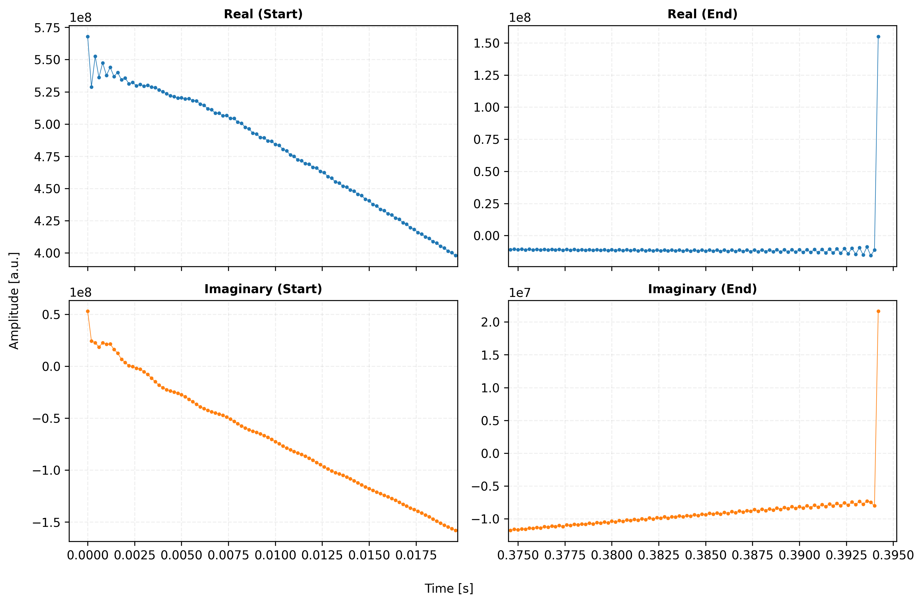
# --- Configuration: Easy Adjustments ---
view_cfg = {
    "zoom_percent": 0.05,    # Window size (5% of total FID)
    "padding_percent": 0.05  # 5% padding relative to the local data range
}

# 1. Transform back to Time Domain
fid_final_apo = fid_final.xmr.apodize_exp(lb=5)

# 2. Setup the 2x2 grid with shared axes for decluttering
# sharex='col' -> Top and Bottom share the same time window
# sharey='row' -> Left and Right share the same amplitude scale
fig, axes = plt.subplots(2, 2, figsize=(11, 7), sharex='col')
(ax_real_start, ax_real_end), (ax_imag_start, ax_imag_end) = axes

# --- Logic: Calculate Time Windows ---
t_coords = fid_final_apo[fid_final_apo.dims[0]]
t_min, t_max = float(t_coords.min()), float(t_coords.max())
t_total = t_max - t_min
window_len = t_total * view_cfg["zoom_percent"]

# Define the data slices for plotting
start_slice = fid_final_apo.sel({fid_final_apo.dims[0]: slice(t_min, t_min + window_len)})
end_slice = fid_final_apo.sel({fid_final_apo.dims[0]: slice(t_max - window_len, t_max)})

# --- Helper to calculate padded limits ---
def get_padded_limits(data, pad_frac):
    d_min, d_max = float(data.min()), float(data.max())
    d_range = d_max - d_min
    padding = (d_range * pad_frac) if d_range > 0 else 0.1
    return d_min - padding, d_max + padding

# --- Execute Plotting ---
# Row 1: Real
start_slice.real.plot(ax=ax_real_start, color="C0", marker='.', markersize=4, linewidth=0.5)
end_slice.real.plot(ax=ax_real_end, color="C0", marker='.', markersize=4, linewidth=0.5)

# Row 2: Imaginary
start_slice.imag.plot(ax=ax_imag_start, color="C1", marker='.', markersize=4, linewidth=0.5)
end_slice.imag.plot(ax=ax_imag_end, color="C1", marker='.', markersize=4, linewidth=0.5)

# --- Apply Dynamic Padding & Scaling ---
# X-Axis Padding (shared by columns)
ax_real_start.set_xlim(t_min - (window_len * view_cfg["padding_percent"]), t_min + window_len)
ax_real_end.set_xlim(t_max - window_len, t_max + (window_len * view_cfg["padding_percent"]))

# Y-Axis Padding (shared by rows)
# We calculate the padding based on the "Start" slice as it's the dominant signal
ax_real_start.set_ylim(get_padded_limits(start_slice.real, view_cfg["padding_percent"]))
ax_imag_start.set_ylim(get_padded_limits(start_slice.imag, view_cfg["padding_percent"]))

# --- Final Decluttering ---
titles = ["Real (Start)", "Real (End)", "Imaginary (Start)", "Imaginary (End)"]
for i, ax in enumerate(axes.flat):
    ax.set_title(titles[i], fontweight='bold', fontsize=10)
    ax.grid(True, alpha=0.2, linestyle='--')

    # Remove xarray's default auto-labels to keep it clean
    ax.set_xlabel('')
    ax.set_ylabel('')

# Add unified labels for the whole figure
fig.text(0.5, 0.02, f'Time [{fid_final_apo.coords[fid_final_apo.dims[0]].attrs.get("units", "s")}]', ha='center')
fig.text(0.04, 0.5, 'Amplitude [a.u.]', va='center', rotation='vertical')

plt.tight_layout(rect=[0.05, 0.05, 1, 1]) # Make room for unified labels
plt.show()